Deep learning
Introduction
Deep learning is machine learning using neural networks with many layers forming a “deep” pipeline. The shift from the “classical” machine learning seen in the previous chapter isn’t just that the models are larger. In classical ML, we choose the model family and select the features ourselves. The model learns from training data but it’s still heavily constrained by our model and feature choices. In deep learning, we still choose an architecture that matches the shape of the data, but the model discovers many of the intermediate features on its own.
Learned features are most useful on data that don’t reduce neatly to regular tables of data. Images, audio, and language are high-dimensional, messy, and full of structure that’s hard to encode by hand. Deep models can uncover patterns that would be painful or impossible to engineer manually. Doing so unlocks amazing new functionality but at the cost of more training data, more compute, more careful training, and less interpretability than the models we’ve seen already.
This chapter treats deep learning as the next step in the machine learning story. We start with neurons and feedforward networks, then move to representation learning, backpropagation, training, and the main architecture families. From there we look at generative models, reinforcement learning, and the practical question of when deep learning is worth the cost. The next chapter builds on this foundation to cover large language models (LLMs) and modern AI systems.
From classical ML to deep learning
Let’s pick up from the machine learning section on feature engineering with our little spam filter example. A classical ML pipeline might represent each email using counts or TF-IDF scores for words, perhaps add a few hand-built features such as whether the sender is known or whether the message contains many links, and then fit logistic regression or Naive Bayes on top. The model makes the final decision, but the representation of the email is mostly our job. The model learns to identify the features we give it, but whether it does a good job of actually identifying spam mostly depends on the quality of the features we provide.
Now change the problem. Suppose we want to recognise cats in photos. How would we go about this with the classical approach? We would come up with a set of features first and then fit a model. That’s exactly how many older systems worked. Vision researchers engineered edge detectors, texture histograms, and keypoint descriptors to try and identify cat-like data. These approaches were often clever and sometimes effective, but they depended heavily on whether the feature engineering exposed the right structure and they were very brittle.
Deep learning automates that process of feature discovery. We still make one high-level design choice up front by picking an architecture that fits the data shape. Our cat example uses two-dimensional images so that suggests convolutional networks. Sequences (e.g. text) suggest recurrent models or transformers. But once that high-level choice is made, much more of the representation is learned automatically via training. Instead of somehow explicitly telling the model which edges, textures, or shapes matter, we give it raw pixels and let it build internal features for itself. The workflow shifts from “design the features carefully” to “design the architecture carefully and let training discover the features.”
That’s why representation learning matters so much. A representation is simply the form in which the data is presented to the model, such as word counts, pixel values, embeddings, or learned hidden features. A classical model usually assumes that the representation is already good enough and focuses on drawing the best boundary or function using that representation. A deep network treats representation building as part of the learning problem. The additional layers of a deep model are where the system itself learns the features it needs.
That doesn’t make deep learning automatically better than classical ML in every situation. On many tabular problems, especially where the columns are already informative and well-structured, classical ML still wins or is at least easier to work with. If you’re pricing insurance from age, vehicle type, claims history, and location, you often already have a sensible feature table, and interpretability is valuable. In that setting, gradient-boosted trees or linear models may still be the right answer. Deep learning shines when the structure of the input is rich but hard to describe manually.
Neural networks aren’t some new-fangled idea. Early models, known as perceptrons, were developed back in the olden days of the 1950s. Researchers jitter-bugged with excitement until disappointment set in when single-layer perceptrons turned out to be severely limited and training deeper networks wasn’t yet feasible. The 1980s brought a mini-revival when multi-layer networks became more practical to train. But the datasets were small (by modern standards), the computers were slow, and the models were temperamental. By the 1990s and early 2000s, many practical problems were better served by support vector machines, tree methods, or carefully engineered features. Neural networks never quite disappeared, but it wasn’t at all obvious that they held much promise.
Several things began to finally line up during the 2000s. First, much more data became available. The web, smartphones, sensors, and digital platforms produced huge labelled and unlabelled datasets as we all mindlessly uploaded our lives on to Facebook and tagged our friends in embarrassing photos. Second, there was far more compute. GPUs, originally built for graphics, turned out to be ideal for the matrix multiplications used by neural networks. Third, a collection of practical ideas made deeper networks trainable enough to use reliably.
The watershed moment came in 2012 when AlexNet won the ImageNet competition. ImageNet is a large-scale image-recognition challenge, and AlexNet won by a margin that made the field pay attention. The result mattered not because one model happened to score well, but because it showed that learned visual representations could surpass the older hand-crafted vision pipeline on a major real task. After that, deep learning spread rapidly through vision, speech, and language. Much of the excitement around “artificial intelligence” in the 2010s was around deep learning systems mastering tasks that had previously been difficult for computers, such as image recognition. That shift also pushed older methods like support vector machines out of the spotlight.
The success of deep learning illustrates what Rich Sutton called the Bitter Lesson (see further reading). Over the long run, many of the biggest gains in ML and AI have come less from carefully hand-crafting domain tricks and more from simple, general methods that can efficiently consume huge amounts of data and compute. We still need good architectures, training objectives, and engineering judgement. But what matters most is whether those methods allow the model to scale well so that it outruns clever feature design by learning the structure directly from raw data. It’s called the “bitter” lesson because of the bitter tears shed by the many researchers who spent years hand-crafting domain-specific improvements only to see general methods, once given enough data and compute, pull ahead. Informally, this is also known as the “GPU go brrrr” theory of artificial intelligence.
It’s important to understand that deep learning didn’t “replace” machine learning. It’s one branch of machine learning that became overwhelmingly strong on certain kinds of data. It extends ideas we already know, such as loss functions, gradient descent, regularisation, and train/validation/test discipline, but it changes where the intelligence in the pipeline lives. In classical ML, we choose the features and then fit the model. There’s still a lot of human judgement and insight going into it. In deep learning, we still choose the broad architecture, but the network learns much of the feature hierarchy for itself. That shift buys capabilities that were difficult or impossible with classical ML.
Neural networks
At the lowest level, a neural network is just a stack of small, parameterised functions. Each layer takes in numbers, transforms them, and passes numbers to the next layer. Stack enough layers together and you can model a wide range of input-output relationships.
Large networks are extremely flexible. That’s the intuition behind universal approximation. With enough capacity, the same general kind of network can imitate an enormous range of input-output mappings. Train one on cat photos and it can become a cat detector. Train a similar network on car photos and it can become a car detector instead. The architecture doesn’t come pre-loaded with either behaviour. Training nudges the weights until one particular behaviour emerges from the huge space of behaviours the network could represent. That doesn’t mean the network will be easy to train or efficient to learn from data, only that the capacity is there in principle.
But that theoretical flexibility is only half the story. A network isn’t useful merely because it could represent the right function in some giant, awkward form. It has to represent it in a way that’s trainable, data-efficient, and computationally reasonable. That’s why architecture matters so much. CNNs make image structure easier to learn. Sequence models make ordered context easier to learn. This is a bit like programming languages. Many are Turing complete, but some are much better fits for particular jobs. In practice, the question isn’t just “is this possible?” but “does this structure make the right solution natural to learn?”
The artificial neuron
The basic building block of the neural network is the artificial neuron. The name is misleading. It’s best thought of not as a tiny brain cell but as a small, adjustable function. A neuron takes several inputs, combines them using weights, adds a bias term, and then passes the result through an activation function:

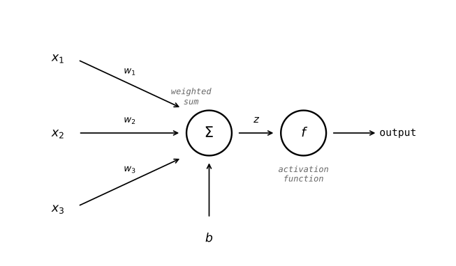
- An artificial neuron
Figure 1 shows the pieces. Each input is scaled by a weight. Those weighted inputs are summed. The bias shifts the result. Then the activation function decides what output to emit. During training, the model adjusts the weights and bias values so that the neuron output becomes useful for the overall task.
Imagine a neuron in a house price model that receives square footage, neighbourhood score, and age of the property. A large positive weight on square footage and a negative weight on age would mean “bigger tends to push my signal up; older tends to push it down. In an image model, the same neuron might instead receive pixel patterns or outputs from earlier feature detectors. The neuron doesn’t know anything about houses or images in a human sense. It only computes a weighted combination and then applies an activation.
The activation function is essential because without it a deep network would collapse into one big linear function. The arguments to the activation function above match the shape of the linear model we saw in the machine learning chapter’s analysis of linear models. In one dimension, linear functions look like straight lines on a graph (hence “linear”). More generally, stacking layers that only do weighted sums still only gives you another linear mapping. If every layer only performed weighted sums, then stacking ten layers would be no more expressive than using a single layer with a combined set of weights. Non-linearity is what allows networks to represent curved decision boundaries, thresholds, and the nested combinations that interesting tasks require.
The most common activation in many networks is ReLU (Rectified Linear Unit), which outputs the input if it’s positive and zero otherwise. It’s almost comically simple, but it works well and helped make deep networks trainable. Earlier networks often used sigmoid or tanh activations. Those squash values into bounded ranges, which is mathematically neat but practically awkward in deep networks because gradients can become very small as they pass through many layers. ReLU avoids much of that problem by keeping a strong gradient on the positive side. There are variants charted in Figure 2. The activation is the point where the network stops being just a mass of linear algebra and becomes capable of learning rich, non-linear behaviour.
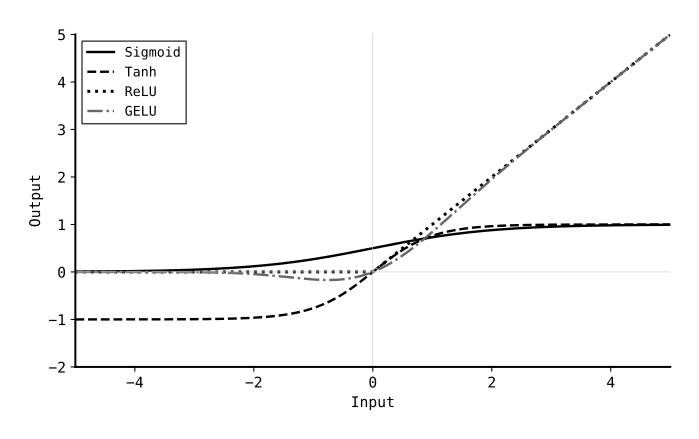
- Common activation functions
Inside the complete chapter
What you’ll learn
- From classical ML to deep learning How learned features replace hand-crafted feature engineering
- Neural networks Neurons, activation functions, backpropagation, and universal approximation
- Deep learning architectures CNNs for vision, RNNs for sequences, and the rise of transformers
- Generative models VAEs, GANs, and diffusion models that produce new data
- Reinforcement learning with deep networks Agents that learn through trial, error, and reward
- Deep learning in practice When deep learning is worth the cost and when classical ML still wins