Machine learning

Introduction

We crossed an important boundary in moving from the previous chapters to here. Much of the book so far has focused on systems whose behaviour is specified explicitly: algorithms, protocols, instruction sets, compilers, and data structures. Machine learning adds a different style of computation. The underlying computer is still a deterministic machine following exact instructions, but the behaviour we care about is now described statistically. Instead of reasoning mainly from logic and formal rules, we start reasoning from data, uncertainty, and probability. The cost is that we often lose some interpretability, and we may lose reproducibility unless the data, randomness, and software environment are carefully controlled, but we gain capabilities such as spam filtering, image recognition, and language understanding that are hard to build with hand-written rules alone.

The umbrella term for this new paradigm is machine learning. Instead of specifying the behaviour entirely with hand-written rules, we provide examples as data and let a learning algorithm fit the pattern. Instead of telling the computer how to do what we want, we show it many data samples and let it figure out the patterns itself. The computer learns from data rather than from explicit instructions.

At first this can sound like magic. How can a computer “learn” anything if it’s still just following instructions? The answer is that the instructions are different. Instead of saying “here is exactly how to do the task”, they say “adjust yourself to get better at the task”. What looks like learning is the result of applying that idea at scale.

Machine learning now powers much of the modern web. Recommendations, fraud detection, search ranking, and spam filtering all use it. For software engineers, some understanding of ML is now part of the job. You may need to integrate an ML-powered feature, decide whether a problem is suitable for ML, or debug why a model is behaving unexpectedly.

The next three chapters build on each other. This chapter lays the foundation. We’ll examine what machine learning is and how it differs from traditional programming. We’ll look at several important algorithms and when to use each. We’ll cover training, evaluation, and the pitfalls that trip up practitioners. We’ll also discuss deployment, monitoring, and the ethical concerns that come with real systems. Throughout the chapter, we’ll keep returning to two running examples: a spam filter for classification and house-price prediction for regression.

One quick note before we begin. Mathematics is unavoidable in machine learning. These algorithms are fundamentally mathematical, and the next three chapters contain more formulas than the rest of the book combined. But my goal here is intuition, not formal derivation. Where a formula appears, I will explain what it means, what it’s doing, and why it matters.

What is machine learning?

Let’s begin with the problem of classifying emails as spam or not spam. In traditional programming, you might write something like Listing 1.

def is_spam(email):
    spam_words = ['viagra', 'lottery', 'winner', 'prince']
    if any(word in email.lower() for word in spam_words):
        return True
    if email.count('!') > 10:
        return True
    if email.sender not in contacts:
        return True
    return False

This works, up to a point. The problem is that spammers adapt. They misspell words (“v1agra”), use images instead of text, and craft more sophisticated messages. You find yourself in an arms race, constantly adding new rules. Worse, the rules interact in complex ways. Emails from unknown senders with lots of exclamation marks may be spam but known senders with them may be legitimate. The ordering above will misclassify messages from particularly excitable correspondents. The rule-based approach becomes unworkably brittle as the number of rules increases.

Take a step back. How did you know that words such as “prince” and “winner” are likely spam? You looked at a set of spam emails and identified common words. You spotted patterns. That’s exactly what the machine learning approach does, as Listing 2 shows.

def train_spam_classifier(labelled_emails):
    features = [extract_features(email) for email in labelled_emails]
    labels = [email.is_spam for email in labelled_emails]
<span class="n">model</span> <span class="o">=</span> <span class="n">SomeMLAlgorithm</span><span class="p">()</span>
<span class="n">model</span><span class="o">.</span><span class="n">fit</span><span class="p">(</span><span class="n">features</span><span class="p">,</span> <span class="n">labels</span><span class="p">)</span>
<span class="k">return</span> <span class="n">model</span>

def is_spam(model, email):
features = extract_features(email)
return model.predict(features)

We’ve replaced explicit rules with a learning process. The fit method examines labelled examples and discovers patterns that distinguish spam from legitimate email. We don’t tell it what patterns to look for. It figures that out from the data. When spammers change tactics, we don’t rewrite rules. We retrain the model on new examples. That’s machine learning in a nutshell: algorithms that improve through exposure to training data. Our job is to provide enough high-quality training data.

Data, models, and learning algorithms

Every machine learning system has three components: data, a model, and a learning algorithm. Problems with any of them will doom your project.

The raw material from which the system learns is data. In our spam example, the data consists of emails with their labels. In our house-price example, it consists of historical properties with features such as size, location, and age paired with the prices they eventually sold for. Data quality matters enormously, far more than any other factor. The old programmer’s adage “garbage in, garbage out” applies with a vengeance. If your training data is biased, incomplete, or incorrectly labelled, your model will learn the wrong patterns. Machine learning can’t magically extract insights that aren’t in the data. We’ll return to this theme repeatedly.

The model is a mathematical structure that captures patterns in the data. You can think of it as a function with adjustable knobs. A very simple model might be a linear equation as in Listing 3. The weights 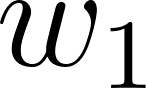, , 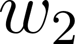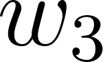(the knobs) are parameters that determine how much each feature contributes to the final score. More sophisticated models have millions or billions of parameters, but the principle is the same. The model is a function, controlled by its parameters, that maps inputs to outputs.

spam_score = w1 * word_count + w2 * exclamation_count + w3 * unknown_sender

The learning algorithm adjusts the model’s parameters to improve performance on the training data. It examines the examples, compares the model’s predictions to the correct answers, and tweaks the parameters to reduce the errors. This process repeats (often millions of times) until the model performs well enough or stops improving.

An analogy might help here. Imagine teaching a child to recognise dogs. You don’t explain the precise rules (“four legs, fur, tail”). Instead, you point at various animals: “dog”, “not a dog”, “dog”, “not a dog”. The child learns by example, often getting it wrong at first (“no, that’s a cat”), but eventually the child learns to recognise dogs, even breeds they’ve never seen. They’ve learned a pattern from examples rather than from explicit rules. Machine learning works similarly, though of course the “learning” is quite different from what happens in a human brain.

Supervised and unsupervised learning

Machine learning problems fall into a few broad categories depending on what kind of data is available and what we’re trying to achieve. In supervised learning, we have labelled examples: inputs paired with the correct outputs. Our spam classifier from earlier is supervised because each training email comes with a label indicating whether it’s spam. The model learns to map inputs to outputs by studying these input-output pairs. Supervised learning is by far the most common type in practice.

Two of the most common supervised problem types are classification and regression. In classification, the model predicts which category an input belongs to: spam or not spam, cat or dog, fraudulent or legitimate. The output is one of a fixed set of possibilities. In regression, it predicts a continuous value: the price of a house, the temperature tomorrow, how long a user will stay on a page. The distinction matters because different algorithms and evaluation approaches apply to each.

In unsupervised learning, we have only inputs without labels. Nobody has told us the correct answers. The goal is to discover structure in the data on our own. One of the most common unsupervised techniques is clustering, which groups similar items together, segmenting customers into market groups, identifying topics in a document collection, or detecting anomalous server behaviour. Unsupervised learning is harder to evaluate because there’s no ground truth to compare against. You might cluster your customers into five groups, but are those the “right” groups? There’s no objective answer. Still, unsupervised learning can reveal patterns that humans wouldn’t have thought to look for.

A third category, reinforcement learning, involves an agent learning through trial and error. The agent takes actions in an environment, receives rewards or penalties, and learns a strategy to maximise cumulative reward. Reinforcement learning has achieved remarkable results in game playing (AlphaGo, Atari games) and robotics, but it’s less commonly encountered in typical web development. I won’t cover it further here because we return to it in the deep learning chapter, where it fits more naturally alongside modern post-training methods. For now, it’s enough to know that modern LLM training pipelines sometimes use reinforcement learning or related post-training methods to improve model behaviour. Generally unsupervised learning and reinforcement learning are a bit heavier on the mathematics.

The training process

The core learning mechanism is deceptively simple. We define a measure of how wrong the model is, then incrementally adjust the parameters to make it less wrong. The measure of wrongness is called the loss function. For a classification problem, the loss might measure how far the predicted probabilities are from the correct answers. For regression, it might measure the average squared difference between predicted and actual values. The loss function gives us a single number summarising how badly the model is doing. Lower is better. Once we have that single number, we find ways to reduce it. As we do so, the model gets better at solving the problem. It learns.

Training means finding parameter values that minimise the loss. For many differentiable models, this becomes an optimisation problem, and a common approach is gradient descent. If you remember calculus, the gradient tells us which direction is “uphill” for each parameter. We go the opposite way, downhill, taking small steps, recalculating the gradient, and repeating. It’s like descending a mountain in thick fog. You can’t see the bottom, but you can feel which way is down and step in that direction. Gradient descent doesn’t search the whole parameter space exhaustively. It starts from the current settings, measures the local slope of the loss surface, and takes a local downhill step opposite the gradient. Repeating that process traces a path through the landscape. The loss function defines a surface with valleys representing good settings and peaks representing bad ones. We’re trying to reach a low valley, ideally the lowest one. The algorithm is shown in Listing 4.

def gradient_descent(model, data, learning_rate, iterations):
    for i in range(iterations):
        predictions = model.predict(data.inputs)
        loss = compute_loss(predictions, data.labels)
        gradients = compute_gradients(loss, model.parameters)
    <span class="c1"># Take a step downhill</span>
    <span class="k">for</span> <span class="n">param</span><span class="p">,</span> <span class="n">grad</span> <span class="ow">in</span> <span class="nb">zip</span><span class="p">(</span><span class="n">model</span><span class="o">.</span><span class="n">parameters</span><span class="p">,</span> <span class="n">gradients</span><span class="p">):</span>
        <span class="n">param</span> <span class="o">-=</span> <span class="n">learning_rate</span> <span class="o">*</span> <span class="n">grad</span>

<span class="k">return</span> <span class="n">model</span>

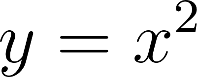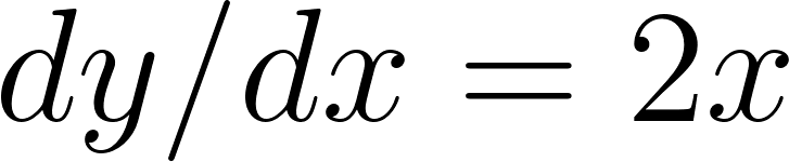The interesting step is compute_gradients. Computers calculate gradients using the chain rule from calculus. For simple functions, we could compute gradients by hand–the derivative (the rate of change) of is . ML models, though, are built by feeding the output of one function into the next, chaining together millions of simple operations. Computing the gradient of the whole chain by hand would be impractical. Happily, calculus has the chain rule, which makes this manageable. Without wanting to get too far into the mathematics, we can work out how to tweak the parameters when the model is differentiable, and modern ML frameworks can handle many of the piecewise operations involved. Modern ML frameworks implement automatic differentiation. You define how inputs flow through the model to produce predictions and loss, and the framework automatically computes gradients by applying the chain rule. Without this, training modern models at scale would be impractical.

Loss functions in depth

The loss function quantifies how wrong the model is. Different problems use different loss functions, and the choice matters. In regression, mean squared error (MSE) is the most common:

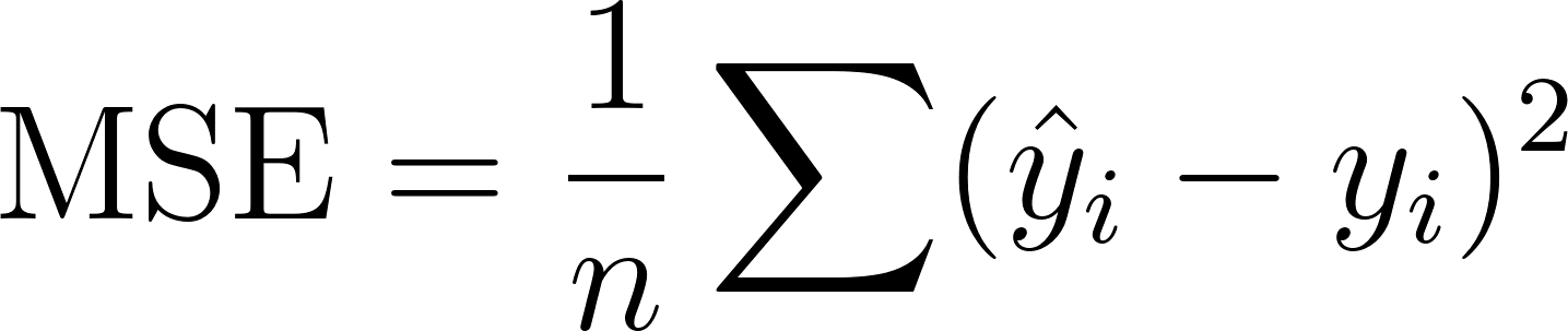
The recipe is in the name. For each prediction 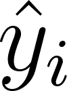, measure how far off it was from the correct answer , square that error, then average over all examples (the means “sum”–you’ll see it a few times). Squaring has several useful properties. It penalises large errors heavily (a prediction off by 10 costs 100, not 10), it’s smooth everywhere (so gradient descent always has a clear direction to follow), and the gradient points directly toward reducing the error. But it’s sensitive to outliers, since one wildly wrong prediction dominates the loss.

If outliers are a concern, mean absolute error (MAE) drops the squaring. Just measure how far off each prediction was, ignore the sign, and average:

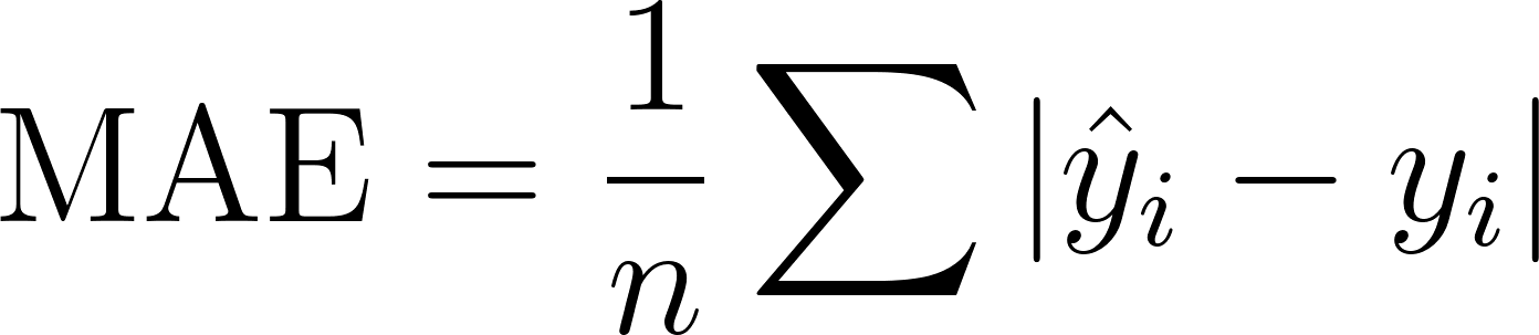
Without squaring, one wildly wrong prediction doesn’t dominate the average, making MAE less sensitive to extreme values. The downside is that the MAE function has a V-shaped bottom rather than a smooth curve, which makes it a little less convenient for gradient-based optimisation.

Classification typically uses cross-entropy loss (also called log loss). The basic idea is that confidently wrong predictions should be punished severely, but tentatively wrong predictions should be punished much less severely. If the model outputs probability that an example is positive, the loss is 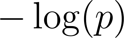when the true label is 1, and 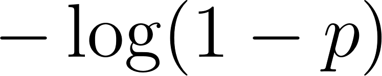when the true label is 0. To see why logarithms matter, imagine a model that predicts 0.999 probability for something that’s actually negative. The loss is . If it had predicted 0.5, the loss would be only . That confident wrong answer costs ten times more than an uncertain one. Cross-entropy therefore rewards models that attach high probability to events that really happen and punishes overconfident mistakes.

In Figure 1 we see how the loss function defines a landscape for a toy model with just two parameters. One axis is , one is , and the height is the loss. Gradient descent follows the slope downward. One challenge is that the landscape can contain local minima, flat regions, and other awkward terrain. Gradient descent follows the slope into a nearby valley, but that valley might not be the best solution. Different starting points may find different valleys, and there’s no guarantee of finding the deepest one (the global minimum). Real models have far more than two parameters, so the same idea lives in a much higher-dimensional space that we can reason about mathematically even though we can no longer picture it directly.