Look at any computer program and you’ll see two things: data and operations on that data. From the computer’s perspective, everything is just a huge sequence of ones and zeroes. It is the programmer who creates meaning by telling the computer how to interpret these ones and zeroes.
In this post, we’ll start off with a quick summary of the distinction between data types and data structures. We’ll then look at one of the most fundamental, but surprisingly interesting, data structures: the array.
Short answer: an array is a contiguous block of memory split into equal-sized slots. If the computer knows the starting address, the size of each item and the index you want, it can jump straight to that item. That one little fact explains why arrays are fast, useful and occasionally annoying.
Here is the quick version before we do the proper explanation:
| operation or feature | what to remember |
|---|---|
| indexing | O(1) |
| insert/delete in the middle | O(n) |
| append to a dynamic array | O(1) on average |
| static array | fixed size |
| dynamic array | resizes by allocating a bigger backing array |
Data types and data structures
A data type defines a set of possible values and the operations that may be performed on those values. Usually a programming language contains a few primitive types such as integers, booleans, dates and so on. These types will have defined operations such as addition for integers or concatenation for strings. Many languages also allow you to define new types (e.g. by defining a class) that build on the primitive types.
A data structure defines a format for organising and storing data. Data structures implement the interfaces specified by data types. Whether a particular data structure is a good implementation of a given data type depends on whether the data structure allows for an efficient implementation of the data type’s operations.
There exists a veritable zoo of data structures out there. I’ve chosen to focus on the array because it is very simple, very important and very useful.
Static arrays
An array is a contiguous block of memory addresses – nothing more. The memory block is conceptually divided into a sequence of locations holding identically sized items. The length, or size, of an array is determined by the total size of the memory block divided by the item size. It indicates how many items can fit into the array. We call these arrays “static” because their size is fixed by the size of the memory block.
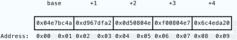
In this example, each item is two bytes long and there are five items. The memory block is therefore ten bytes long and the array has length five.
Note that in the diagram above I use black borders to delineate each item. In memory, the bytes are all adjacent to each other so the array would actually look like this:
0x04e7bc4ad967dfa20d50804ef00804e76c4eda0
The array’s elements have to be the same size so that the computer can know where the bits making up one item end and the bits making up another item begin. An array is therefore associated with the particular data type that it contains.
Now that we know how an array structures its data, let’s consider which operations it can perform efficiently. Well, we can very easily iterate through the array by pointing a counter to the base address and repeatedly incrementing it by the item size. We can even jump directly to any item (i.e. index it) by multiplying the item’s position by the item size and adding that to the base address. We’re able to do this because the structure of the array allows us to work out the location of any item, provided we know the base address, the item size and the desired item’s position within the array.
The strength of the array is its speed. Iteration only requires incrementing a counter and indexing to any item can be done in constant time. No matter how far away the desired item is, we can always jump directly to it just by computing its address. The simplicity of the array is also its main limitation. If we want to add or delete an element somewhere in the middle of the array, we’ll need to move the existing items around.
Worse, there is nothing that marks the end of the array and so there is no way for the computer to know when it’s exceeded the bounds of the data. In C, a variable holding an array actually just holds the array’s base address. This means that the size of the array has to be stored in a separate variable and passed around with the array. The programmer is responsible for correctly updating the size when necessary. If you mistakenly give the computer an incorrect value, it will blithely iterate past the final item, possibly overwriting any values stored in those locations. This is known as a buffer overflow and is a major source of often very serious bugs.
A second limitation of static arrays is that, as already mentioned, their size is fixed. What happens when we want to add more items than the array has space for? You might think that we could just make the array bigger by allocating more memory at the end of the memory block. But this is often not possible because the adjacent memory addresses might already be in use. Instead, the computer has to allocate a new, unused block of sufficient size and copy over all of the existing items.
Get the free 45-page CS roadmap
Subscribe and I'll send you a free, 45-page roadmap through computer science — what to learn, in what order, and what to skip — plus the occasional CS deep dive.
No spam. Unsubscribe anytime.
Dynamic arrays
Manually handling array sizes and reallocating blocks in C is generally seen as a bit of a pain. More modern programming languages usually provide a slightly different, more convenient data structure known as the dynamic array.
A dynamic array holds a static array in a data structure along with the current size and the total capacity (i.e. including unused space), thus preventing out-of-bounds operations and removing the need to store the size in a separate variable. Even better, dynamic arrays automatically resize when they get filled up. The upshot is that we can add as many items as we want without having to worry about the size of the array.
In many languages, it’s hard to dig into the inner workings of a dynamic array. This is by design: the whole point of dynamic arrays is to take this responsibility away from the programmer. Go offers an interesting intermediate point between static and dynamic arrays. Go has C-style, static arrays but builds on top of them a dynamic array known as the slice, defined in the Go source code (runtime/slice.go) as a wrapper around an array:
type slice struct {
        array unsafe.Pointer
        len   int
        cap   int
}
“Pointer” here means a value that is the address of another value. It points to the value’s location. The slice therefore doesn’t actually contain the array; it just knows where the array is located. As well as the address of its underlying array, the slice tracks the len, the number of items in the array, and the cap, the total capacity of the array.
Since a slice is just a struct, Go lets us inspect all of these properties just like any other value. Let’s observe it in action:
slice := []byte{1, 2, 3}
array := [3]byte{47}
First, we define a byte slice and initialise it with three values. Immediately afterwards, we define a (static) byte array of size three but with only one initial value. Let’s print some information about the slice:
fmt.Printf("Slice %#v has length: %d and capacity: %d\n",
        slice, len(slice), cap(slice))
fmt.Printf("Slice item addresses: [%#p, %#p, %#p]\n\n",
        &slice[0], &slice[1], &slice[2])

// Output:
Slice []byte{0x1, 0x2, 0x3} has length: 3 and capacity: 3
Slice item addresses: [c000086000, c000086001, c000086002]
Note that, in this case, the size of the slice and its capacity are the same. That means it has no more space for new items. And here’s some information about the array:
fmt.Printf("Array %#v has length: %d\n", array, len(array))
fmt.Printf("Array address: %#p\n\n", &array)

// Output:
Array [3]byte{0x2f, 0x0, 0x0} has length: 3
Array address: c000086003
Even though array only contains one actual value, we defined it to have length three so space for two more has already been allocated.
Notice that the items held by slice are all adjacent to each other in memory and the address of array comes directly after. That means there is no empty space between the two variables. What do we expect to happen when we append another item to the slice? There won’t be room for a fourth item and we can’t just expand the underlying array because the memory address is already occupied. We therefore expect that the slice will allocate a new, bigger memory block and move all the existing items:
slice = append(slice, 4)
fmt.Printf("Slice %#v has length: %d and capacity: %d\n",
           slice, len(slice), cap(slice))
fmt.Printf("Slice item addresses: [%#p, %#p, %#p, %#p]\n",
           &slice[0], &slice[1], &slice[2], &slice[3])

// Output
Slice []byte{0x1, 0x2, 0x3, 0x4} has length: 4 and capacity: 8
Slice item addresses: [c000086030, c000086031, c000086032, c000086033]
The items all have new addresses because they have been reallocated to a different block of memory. The slice allocates a bit of extra space, raising the capacity to 8, to allow more items to be appended without having to immediately resize again. It’s common for dynamic arrays to double their capacity whenever they reallocate because reallocations are expensive and it is better to possibly have some unused capacity that to perform repeated reallocations.
Array vs linked list
Arrays are great when you want simple storage, fast indexing and efficient iteration. Because the elements sit next to each other in memory, the computer can calculate addresses directly and the hardware has a decent chance of keeping nearby values ready in cache. This is one of those places where the tidy abstract data structure and the messy physical machine happen to get along rather nicely.
Linked lists make a different trade-off. Each item points to the next item, so the values do not need to sit in one contiguous block. That means insertion and deletion can be cheap if you already have a reference to the right node. The cost is that you lose direct indexing. To find the hundredth item, you have to start walking from the beginning and count like some sort of very patient machine.
The algorithms and data structures chapter goes through the wider trade-offs. For now, the important point is that an array is not “better” than a linked list in the abstract. It is better when its strengths match the operations you actually need.
Conclusion
To sum up, arrays are contiguous blocks of memory holding identically sized elements, making it possible to immediately access any element. Adding an element somewhere in the middle involves shuffling every subsequent item along to make room. Deleting an item entails shuffling in the other direction to fill the gap. Adding an element at the end should be immediate, unless the array is already full and the whole thing needs to be reallocated. This gives us the following performance summary, using big-O notation:
| operation | performance |
|---|---|
| index | O(1) |
| insert/delete at beginning | O(n) |
| insert/delete at middle | O(n) |
| append | O(1) average |
The disadvantage of static arrays is that expanding the array involves allocating a new memory block and copying everything over. Dynamic arrays keep track of their capacity and will automatically reallocate when necessary. This makes things much easier for the programmer and, if we average out the occasional cost of reallocation, keeps things pretty performant.
For situations where you don’t need to index items but want to efficiently add and remove items at the beginning or middle, a better data structure might be the linked list.
FAQ
A few quick answers, since arrays are simple enough to describe in a sentence and annoying enough to deserve caveats.
How does an array work?
An array stores equal-sized elements next to each other in memory. Each element has a numeric position, or index, which the computer can use to calculate where that element lives.
What is a dynamic array?
A dynamic array is a more convenient wrapper around a fixed-size backing array. It tracks its current length and total capacity, then allocates a bigger backing array and copies values over when it runs out of room. This is why appending is usually cheap, but occasionally surprisingly expensive.
What is the difference between an array and a linked list?
An array stores elements contiguously, so indexing is fast. A linked list stores nodes connected by pointers, so inserting or deleting can be cheap if you already have the right node, but finding the nth item means walking through the list one step at a time.
What is the difference between a static and dynamic array?
A static array has a fixed size. If you need more room, you have to allocate a new block and copy the old values over. A dynamic array wraps that static array with length and capacity information, then does the resizing for you when necessary.
Get the free 45-page CS roadmap
Subscribe and I'll send you a free, 45-page roadmap through computer science — what to learn, in what order, and what to skip — plus the occasional CS deep dive.
No spam. Unsubscribe anytime.