How my 2yo taught me constraint solving

Reading on email? The visualisations will work better in browser.

My son is two years old, which means he has an Apollonian will to power and loves all kinds of mechanised transportation and earthworks machinery. His particular joy is “playing choo-choo” with a Brio wooden train set. Since he likes me to be involved, but I am expressly NOT permitted to touch the trains, I amuse myself by building interesting track layouts.

After a long while, I began to think more systematically about Brio. The pieces are clearly designed to fit together into shapes, so what’s the underlying structure in the design? Given out set of pieces, what is the most elaborate layout I can build?

I don’t have a formal maths background, but I could see that this was an interesting algorithms problem lying on the floor in front of me. As I explored this, my son demonstrated a hitherto undetected expertise in constraint solving. The rest of this post is a lightly editorialised account of what he told me.

The Brio system

Brio is a wooden train toy for kids but has been documented in depth by particularly interested adults. I first turned to the unofficial Brio track guide, which gives every piece a letter code and a measurement. A is the 144 mm medium straight. A1 and A2 are 108 mm and 54 mm variants. E is the standard curve, an eighth of a circle, measuring just over 182 mm on the inner edge and 222 mm on the outer. Eight of those 45-degree curves therefore enclose a circle about 40 cm across. Most pieces can be flipped over, so a curve can bend left or right depending on how you arrange it.

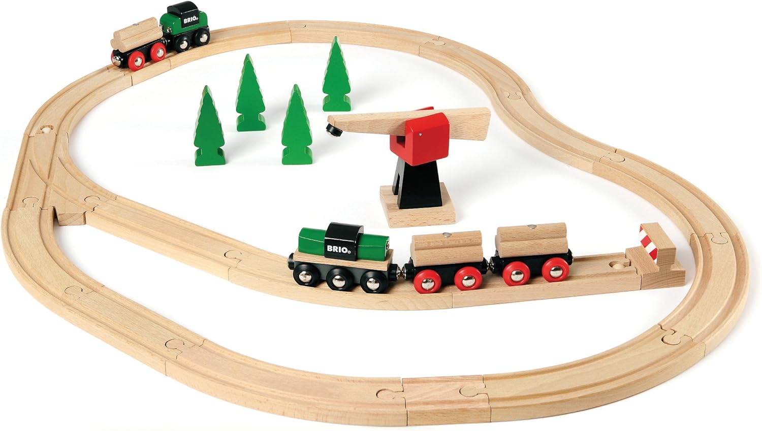
You get ramps and bridges too, but let’s ignore them and treat the system as two dimensional for simplicity. This suits me because the bridges are quite rickety and my son keeps knocking them over, so I try to hide those pieces.

First, make the track close

One morning I begin by putting eight curves together to form a circle.

“Circle!” my son cheers.

Good! Reading Shapes with Thomas the Tank Engine and his Friends for hundreds of times has paid off.

But this is the simplest possible closed Brio loop. Where do we go from here? What sounds fun to me is to take a set of track pieces and find whether every one of them can be arranged in a closed layout (i.e. with every connector paired up).

This post features visualisations powered by three solvers of increasing sophistication. Figures one to four run a backtracking search, figure five uses constraint solving, and figure six uses a SAT solver.

The backtracking search builds the track the way a toddler would: put down a piece, look at the open connectors, try another piece, back up when something doesn’t fit. Here’s how we’d make a loop:

Actually, my son throws the choo-choo in a rage when the track doesn’t fit, but the solver performs recursive backtracking instead, a common way to explore a search space for those with self-control.

The open connectors form a task list. The solver works on just one of them at a time, trying every piece and orientation that fits there and recursing into each. When a branch hits a dead end — no piece that can fit, or every piece used up while connectors are still open — it backs up to the last connector that still had options. The track only counts as closed once no connectors remain open and every piece in the set has been placed. Closing early with pieces still spare is treated as another dead end to back out of. In Python-style pseudocode, it would look something like:

def search(open_connectors, unused_pieces, layout):
    if not open_connectors:
        return layout if not unused_pieces else None

    connector = open_connectors[0]
    for piece in unused_pieces:
        for port in piece.ports:
            placement = mate(piece, port, connector)
            if collides(placement):
                continue
            found = search(update(open_connectors, placement),
                            unused_pieces - piece,
                            layout + placement)
            if found is not None:
                return found
    return None

With eight E curves, the problem is pretty trivial as long as you lay every curve facing the same direction. The solver doesn’t know that, though. If you step through the figure above and watch the “states explored” count, it will jump up very quickly. That’s because the search first tries a curve bending the wrong way, following that dead end until it runs out of pieces without ever closing, then backing out and laying the curve that actually works. The “states” count tracks that whole wasted subtree.

“More, Dada!” he says.

Making the track bigger

So I make the track bigger by splitting the circle and adding some parallel straight sections on opposite sides.

“Oval!” I say, as if I’ve discovered geometry.

“No, Dada, oblong,” he says, pointing at the straight sections.

I stare. He’s right. His nursery worker had said he seemed quick. Perhaps the fees were worth it after all.

Trying to quickly recover authority, I consider the algorithmic impacts. Adding two straight pieces dramatically increases the number of possible states.

The obvious approach uses a greedy algorithm: take the first piece that fits, keep going, and never look back. But a piece can fit in one place and still make it impossible to ever close the track. The straight pieces in particular only work in a few positions. A greedy run would use one of them in the wrong place, get stuck, and have nothing left to do about it. So we want the ability to backtrack from dead ends, unwinding the placements we’ve made and trying a new piece.

I explain this gently. “Exponential, Dada,” he nods.

Indeed. Every open connector can be continued by any piece that fits it, so the number of partial layouts grows exponentially with the number of pieces, very roughly O(b^n) for a branching factor b and n pieces. This figure has only two more pieces than the previous circle, but it tries 1,930 states against the circle’s 254. That’s about eight times as many states for two extra pieces.

So if it’s an algorithm with exponential running time, how is it running reasonably quickly in your browser? At this size, it doesn’t need to be clever: a couple of thousand states is nothing for a laptop to chew through, so plain exhaustive backtracking — trying every piece and port in a fixed order, no shortcuts, no cleverness — finishes in milliseconds. That won’t stay true forever. The worst case is still exponential, and we’ll hit the wall soon.

Anyway, circles and oblongs or ellipses or ovals or whatever you call them are boring. It’s not hard to make a bigger one but the trains just go round the same. We need crossings and branches to make things interesting.

Crossings add branching points

My son picks up a crossing piece (H3). It’s made from two overlapping circles so a train rolling through can stay on its groove or switch to the other line.

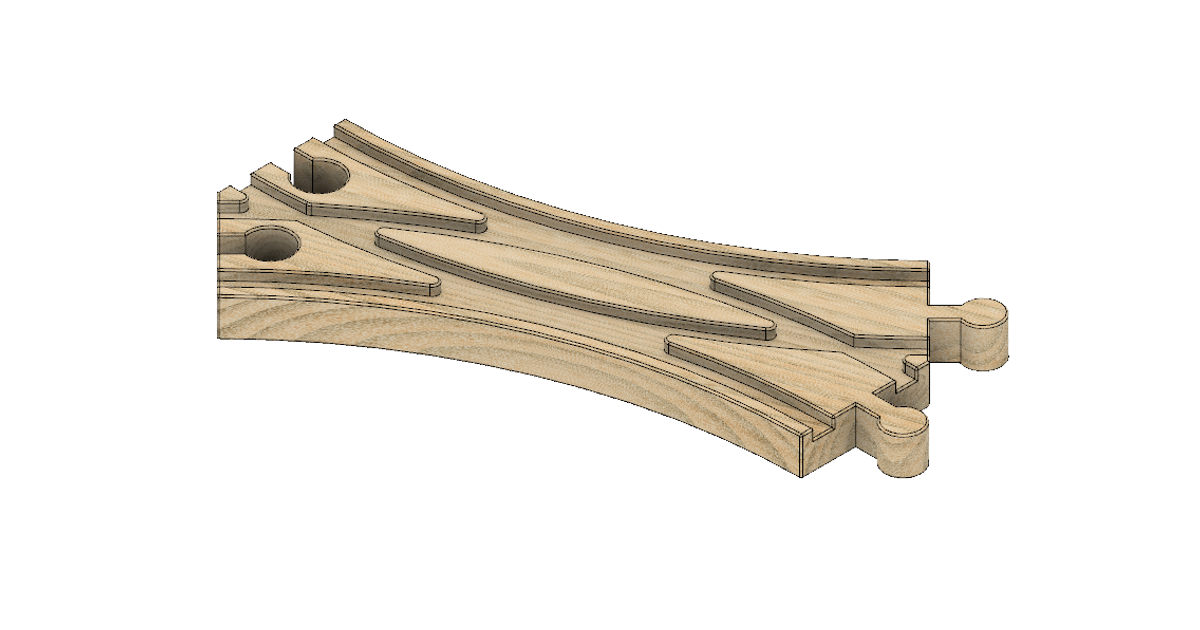
Now we have branching points! I show my son. “Look, we’ve got a crossing piece here.”

“Graph with two cycles!” he beams.

I melt with pride. My own little computer scientist! A future terror of Hacker News comment sections!

As we saw in the graphs section of The Computer Science Book, a graph is the mathematical term for points joined by lines (the points are vertices, the lines are edges), and a cycle is any route through the graph that comes back to where it started. Every track piece up to now had two connectors, so the track was like a single thread, going from one end and round to the other. One cycle, if it formed a closed loop. The crossing has four connectors, so placing it opens three connectors at once and the search itself starts to branch. The data model had to change from this:

piece = geometric move

to this:

piece = connectors + geometry + internal grooves

The search algorithm didn’t change but it is now searching over a more complex space.

The goal, remember, is to check whether every piece in the set — crossing included — fits into one closed network. And it does. Two full circles joined through the crossing, every connector paired, and the train threading both grooves on a single lap.

An interesting sidenote is collision detection. Initially, I added this as a constraint because the solver kept trying to cheat by laying pieces over the top of each other. I added it for correctness but the extra constraint also helped speed up the search. More constraints reduce the size of the search space that has to be explored.

Branches turn the loops into a network

The L branch is a straight and a curve sharing one connector. The choo-choo can carry on straight or peel off around the curve. The M is its mirror image.

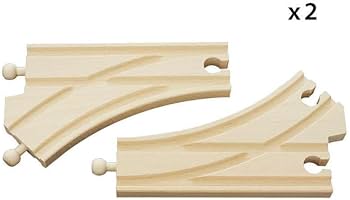
The solver can now find more interesting layouts. It creates an inner loop between the two branches so that there’s an oblong on the outside, a circle on the inside, and every one of the branches’ three connectors is paired.

“Dada! Degree three. No Euler circuit.”

After consulting with ChatGPT, I understand what my son means.

Degree just counts how many track-ends meet at a point, so the crossing (four connectors) is degree four and the branch (three connectors) is degree three. As my son explained, graph theorists call the track shape a theta graph, because it looks like the letter θ. Euler proved in 1736 that a vertex of odd degree means that single lap cannot cover every piece of track exactly once. (Euler had bridges in mind, not wooden trains, but the beauty of maths is that the insight transfers). The crossing has an even degree and that means a choo-choo can follow the full figure-of-eight in a single lap. When we use branches, the track is fully closed but the train can’t cover the full path in one lap.

Turning it into a constraint problem

My track layouts have stopped impressing my son. Desperate, I try to make the most impressive track yet: lots of crossings, lots of branches, the whole works.

I tip the whole set of pieces out onto the floor and try to make a super duper complex layout. I fail pretty badly. I get so far and then find that pieces are just too far apart to connect. The search space is exponential in the number of pieces, and here I am adding pieces.

My son watches me with an implacable stare before finally sighing with the heaviness unique to two-year-olds.

“Dada,” he says, “this is a constraint satisfaction problem, silly billy!”

“What do you mean?” I ask, not without some frustration because I dimly suspect he has a point.

“Variables are the open connectors. Domain is the pieces that still fit. Constraints say every connector pairs!”

Of course! How had I missed this? In normal language, a constraint satisfaction problem is what you get when you can say three things:

• what choices are being made
• what each choice is allowed to be
• which choices aren’t allowed to live together

Sudoku, for example, is basically a constraint satisfaction game. No row, column, or box can repeat a digit, so you have to work out where they can fit. This is what constraint solvers do.

Translated to Brio, the choices are where the pieces go. The allowed values are the positions, rotations, and flips they can take. The constraints are the physical rules we’ve been gathering: connectors have to meet, track can’t pass through track, etc.

If you stop to think about how backtracking works, it seems ridiculously wasteful in two ways. It has no foresight: it only discovers a branch is doomed by running out of pieces, long after the placement that doomed it. And it has no aim: when it fails, it undoes its most recent placement and tries the next, even when the real mistake was made ten pieces ago and we should try a whole new direction.

“You need propagation,” my son says, not looking up from his blocks. “And backjumping.”

I hadn’t, in fact, known that I needed propagation and backjumping.

In the constraint solver, the track still grows one open connector at a time, but each open connector now keeps a shortlist of the piece-and-port combinations that could legally go there. That shortlist is its domain.

Forward checking keeps the shortlists up to date. Whenever a piece is laid, the solver crosses off any option that would now collide with the layout, or that needs a piece we’ve already used. If a connector’s shortlist empties, the branch can never close, so the solver gives up on it straight away. Conflict-directed backjumping decides how far to unwind. Rather than undoing one piece at a time, it works out which earlier placement caused the failure and jumps straight back there.

I gave it the same twelve pieces as figure four, ten curves and the two branches, so I could compare it directly against plain backtracking on a problem we’ve already measured.

Unexpectedly, my first version made things worse. It tried 853,186 states against figure four’s 434,791, nearly twice as many. I didn’t believe it, so I ran it on a dozen other sets of pieces, and forward checking made the search slower every time.

Why is this? Does my 2yo not know very much about constraint solving after all?

The reason comes down to what forward checking can and can’t see. It only abandons a branch when some connector’s shortlist empties, and that requires laying a piece that rules out every option at that one connector. But Brio dead ends are hardly ever local. Pretty much any piece fits almost any open connector, so the shortlists stay full right up until the pieces run out. What actually kills a branch is when the remaining pieces can’t supply enough connectors to pair off everything still open, or the open ends have drifted further apart than anything left in the box could bridge. So forward checking only detects the problem at exactly the same moment plain backtracking does, making it not worth the effort.

“You’re checking connectors, Dada,” my son sighs. “Check all the pieces.”

He means a global constraint, one that looks at the whole layout rather than any single connector. After every placement, the solver now checks two whole-layout facts directly: are there enough connectors left to pair off everything still open, and can the remaining pieces reach across the gaps? If either answer is no, the layout can never close, so the branch is abandoned immediately.

This time it works. Same pieces and same rules as figure four, but the search now takes 53,484 states, about an eighth of what plain backtracking needed. The global check cut the search by anywhere from two to nine times on most other sets of pieces I measured, but not all of them. On one set, mixing straights with both branches, this solver is about ten times slower than plain backtracking. The extra checks usually save more work than they cost, but there’s no guarantee.

One additional weakness remains. When this solver backjumps, it forgets the failure as soon as it lands, so if the same dead end comes up in a different part of the search it gets rediscovered from scratch. What I want is a solver that remembers a failure as a rule, so the same mistake is forbidden everywhere else.

Something else is bothering me too. Both of these searches only answer yes or no for one exact set of pieces. If I want the most complex layout, I’m still the one guessing which pieces to try, one set at a time.

“I wonder how I can make the best layout,” I ask myself.

“Let the solver choose the pieces, Dada,” he says softly. I can sense he is disappointed in me.

Handing it to a SAT solver

Initially I thought of the track layout problem as a graph theory question, but that was only true after I’d already solved it. Once the pieces are down, yes, we can describe the layout as a graph. Before that there’s no graph, just a pile of pieces on the living room floor and a small child stumbling all over them.

In fact, the problem is closer to a tiling problem where we choose pieces, place them, and make sure nothing overlaps. We aren’t selecting edges from an existing graph. We’re placing pieces to create the edges.

My son demonstrates this by sorting pieces into piles. “Curves here. Big ones here. Baby ones here.” Then he lines four curves into a square-ish blob and says, “Like polyominoes.”

“Polly what?”

“Polyominoes, Dada. So we can use SAT solver,” he mumbles without looking up at me. I am no longer the father he thought he had.

Polyominoes are Tetris-like shapes and fitting a set of them together without gaps or overlaps is a classic tiling puzzle. Tiling is also one of the standard problems given to SAT solvers, which is the connection he’d made. Brio is the same kind of problem, but with curved pieces instead of square ones, placed so that nothing collides.

Of course! I smack my forehead. “Converting the task to a SAT problem will make it much easier to solve!” I say. He nods.

The Boolean satisfiability problem takes a formula with boolean variables (e.g. a && (b || !c)) and asks whether there is a set of variable assignments that evaluates the formula to true. For example, a := true, b := true, c := false would evaluate that formula to true. The formula is satisfiable if there is at least one valid assignment. The Boolean satisfiablility problem was the first to be proved NP-complete, so all problems in NP can be reduced to Bool SAT (read the theory of computation chapter if I’ve just bewildered you).

The practical upshot for us is that lots of effort has gone into optimising SAT solvers, so even though it’s still NP-complete we can leverage them to quickly find optimal layouts. But a SAT solver only understands true and false, so every possible placement has to become its own yes/no question like “is this piece used, at this spot, at this angle?” The solver needs all of these questions written down before it starts, which means listing every position a piece could ever occupy.

In a tiling puzzle, that list is easy because the positions form a grid, so there’s a fixed set of positions. Brio doesn’t work like that. As every two year old knows, if something doesn’t fit, you can just jam it in. The Brio designers wisely allowed for this behaviour with the (somewhat grandly named) vrio flex system. Connector pegs are slightly smaller than connector holes, giving each piece a few millimetres of wiggle room. Brio pieces don’t snap to a grid.

With a fixed set of pieces the reachable positions are still finite, so in principle you could list them. However, the only way to find one is to build a layout that reaches it, and finding every last one means walking the whole search space, which is the same exponential search we’re trying to avoid.

My way around this was to cheat. Before the SAT solver runs, a search builds layouts from a range of starting sets of pieces and records every connector position it visits along the way. These recorded positions become the only spots the SAT solver is allowed to build on. This approach limits what the SAT solver’s answers mean. A “no” doesn’t mean no closed layout exists anywhere, only that none exists using the recorded positions. A search that ran for longer might find one more position that changes the answer.

Each placement that lands on the collected positions is one boolean variable:

x[placement] = true if this exact piece, here, in this orientation, is used

The rules become clauses. A clause is the only kind of statement a SAT solver accepts. It says that at least one claim from a list has to hold, where each claim is either “use this placement” or “don’t use that one”. Everything the track needs has to be phrased that way:

each used port mates exactly one opposing port
no two crossing placements are both used
at most as many of each junction as the inputs allow
as many junctions as possible, demand relaxed until it closes

Give these clauses to the solver and it looks for a true/false assignment that satisfies every clause at once. If the solver says no, it has proved there’s no possible assignment using the variables it was given. It runs on the same five-second clock as the other two solvers, although the runs on this page finish comfortably inside it.

The bit I got stuck on was the connectivity requirement. “There’s no single clause for ‘all of this fits in one layout’,” I said. “How can I give that to a SAT solver?”

My son talked me through a clever approach using loops. Since there’s no single clause for “all of this fits in one layout”, a set of local rules can still produce two separate railways. In a loop, we solve once and if the answer comes back as two separate railways, add a clause forbidding that exact combination and solve again, counterexample by counterexample, until the layout comes back connected. My son argued that maximising branch points works the same way. Ask for a lot of junctions, and if that’s unsatisfiable, ask for one fewer, until something closes.

The connectivity loop looked like a dodgy hack to me at first, but my son assured me that integer-programming solvers handle the travelling salesman problem the same way, banning each disconnected sub-tour as it appears. Verification people call the general pattern counterexample-guided refinement, apparently.

The SAT solver itself is doing something clever underneath. It guesses a variable, then propagates everything the clauses imply. When it hits a contradiction, it works out which guesses caused it and writes that mistake down as a new clause, so no later branch is allowed to repeat it. Then the solver jumps back only as far as the new clause demands and carries on, restarting now and then but keeping everything it has learned. My son casually referred to this as conflict-driven clause learning or CDCL.

SAT isn’t necessarily faster than the searches we’ve already seen. On this many pieces it’s actually slower and uses far more memory. So why bother? Backtracking and CSP answer yes/no for one exact set of pieces. The SAT solver can take a given number of pieces and find the most complex layout possible, even if that involves leaving some pieces out.

The number inputs in the visualisation above are upper limits, not hard requirements. Every run asks for the most junctions the collected positions can hold and reduces only when that’s been proved impossible. Raise the branches to two of each and the solver builds a seven-junction network of forty-nine pieces. Set the crossings to zero instead and it rebuilds the network around the branches alone.

On a small, fixed set of pieces, backtracking and CSP answer within the five-second budget. They’re fast, simple, and cheap on memory, but neither can tell you what to leave out, because neither is allowed to leave anything out. SAT holds every candidate placement in memory at once, and a rule learned from one dead end is remembered for everywhere in the search, not just the branch where it was found. That costs memory and speed, but it lets the solver select pieces rather than just verify them.

“Dada, real planners use SAT and its relatives for timetabling, chip layout, and routing for the same reason.”

What I learned

Chastened, I lay out the wooden track pieces according to the SAT solver’s output. I had thought Brio would be a chance to show my son some basic shapes, but it turned out his nursery had him on an accelerated algorithms programme and he schooled me. (That explains how he’s so good at packing his backpack at home time.)

My real mistake wasn’t the algorithm but assuming there was one question. “Does this exact set of pieces close?” and “which pieces make the most complex network?” are different questions, and I’d been trying to answer the second with tools built for the first.

Recursive backtracking promises the least: exponential worst case and no memory between dead ends. In exchange, it’s simple, needs almost no memory, and on the sizes in this post feels instant.

The CSP solver keeps the same question but searches more intelligently. The useful part was the feasibility check on the whole layout, because this puzzle’s failure states are mostly global facts that no local check can spot early. The takeaway here is that constraint solving doesn’t magically improve a search. It requires finding useful constraints that drastically reduce the possible search space.

The SAT solver changes the question, not just the search. Clause learning gives it the permanent memory that CSP’s backjumping lacks, so one dead end rules out the same mistake everywhere. The costs are memory, speed, and scope: it holds every placement and every learned clause at once, it takes seconds where the other two take milliseconds, and its proofs only cover the input space it’s given.