Alan Turing (1912-1954) is the founder of computer science. In a single paper from 1936, On computable numbers, with an application to the Entscheidungsproblem, Turing presented the first precise definition of computation. He did this by devising an imaginary computational device, which he called an “automatic machine”, and proving that it was capable of carrying out any computation.
In doing so, Turing proved that his automatic machine was equivalent to computation itself. By exploring what his machine could do, Turing could analyse the capabilities and properties of computation. Automatic machines are nowadays known as Turing machines in recognition of this seminal achievement.
But Turing wasn’t done yet! In the same paper, he went on to demonstrate that there were situations in which a Turing machine would be unable to compute a result. This is known as the halting problem because the machine would run forever instead of halting operation. Since he had already shown that the Turing machine defined computation, the halting problem demonstrated that some things were uncomputable – that’s what’s meant by “an application to the Entscheidungsproblem” in the paper’s title. I think computer science is possibly unique in having both its potential and its limitations set out so clearly in its founding paper.
In this blog post, we’ll focus on the definition of Turing machines and Turing’s proof that they are the most powerful computational model. I’ll cover the halting problem in its own article later.
What do we mean by “computation”?
Before Turing, “computation” had a rather vague definition. Computing a value meant generating a result by methodically, or might we say mechanically, applying a defined sequence of operations. No special insight or ingenuity is required. The word “computer” existed but it actually referred to a person who manually computed numbers using pen and paper.

The problem was that this definition was imprecise (what does “insight” mean?) and couldn’t be analysed mathematically. It was not clear what was computable and what was not. Mathematicians were particularly keen to know whether they could devise some mechanical procedure to compute interesting mathematical theorems so that they didn’t have to sit around finding theorems themselves. Turing set out to solve this question by precisely defining computation and then probing its limits.
In his paper, Turing used the example of a human computer as his starting point:
“Computing is normally done by writing certain symbols on paper. We may suppose this paper is divided into squares like a child’s arithmetic book…I assume then that the computation is carried out…on a tape divided into squares. I shall also suppose that the number of symbols which may be printed is finite.
“The behavior of the computer at any moment is determined by the symbols which he is observing, and his “state of mind” at that moment. We may suppose that there is a bound to the number of symbols or squares which the computer can observe at one moment. If he wishes to observe more, he must use successive observations. We will also suppose that the number of states of mind which need be taken into account is finite.
Turing narrows down what the human computer is permitted to do at each step of the computation:
- Modify the currently observed symbol and possibly change his state of mind, or
- Observe a different symbol and possibly change his state of mind
Clearly, “state of mind” is doing a lot of work here. At first glance, it might seem absurd to reduce someone’s mental state to a single value. It does make sense, however, if we think of “state of mind” as more like the current state of the computation. For example, if I asked you to laboriously write out how you would compute (2 * 3) + (5 * 5), you might write something like this:
(2 * 3) + (5 * 5)(2 + 2 + 2) + (5 * 5)6 + (5 * 5)6 + (5 + 5 + 5 + 5 + 5)6 + 2531
Each step records a particular state of mind as you progress through the computation. At any step, you could give the half-finished computation to someone else and they could use your notes to pick up from where you had left off. Their overall state of mind will obviously not be exactly the same as yours, but enough information is conveyed to resume the computation at the correct point.
The written notes above are a physical record of the current computational state. Turing realised that a machine could perform computation by encoding its progress in its structure.
Defining the Turing machine
A Turing machine is not a physical device but a description of a mathematical object. Turing’s aim was to come up with a formal, mathematical description of the simplest possible machine capable of arbitrary computation. Keeping things simple would make it easier to analyse its capabilities using logical proofs.
A Turing machine consists of a control unit that holds all the possible states and tracks the current state. The control unit has a “tape head” that can read instruction symbols printed on an infinitely long tape. The control unit can move the tape head back and forth along the tape and update the currently observed symbol. The tape acts as both the machine’s working memory, allowing it to record intermediate steps, and as an means to read and output data.
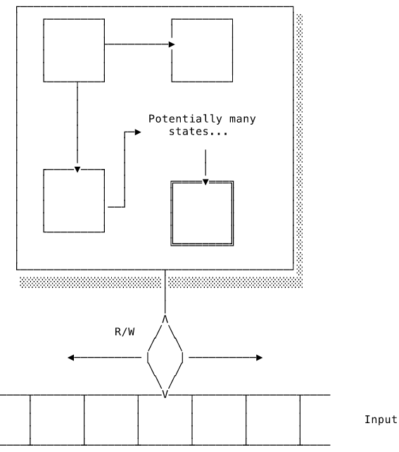
The definition of the machine determines the set of possible states, the set of valid instruction symbols and how the machine should respond to each instruction. The machine starts in an initial state and with the tape head at the beginning of the symbols. At each step of the computation, the machine reads the current value under the tape head, optionally updates the current state, writes a value to the current tape position and then moves a single step to the left or right.
We can express this more succinctly by defining what is known as a transition function:
shiftDirection :: Left | Right
transition :: (currentState, currentTapeValue) -> (newState, newTapeValue, shiftDirection)
Note that newTapeValue might be identical to currentTapeValue, resulting in no overall change to the tape.
The machine terminates, or halts its operation, if it moves into a success or failure state. To compute a number, for instance, the machine would write the number’s digits on to the tape and then halt.
And that’s it! Perhaps a little underwhelming? It seems doubtful that such a simple machine could be capable of any computation. Let’s see what Turing has to say about this.
Get the free 45-page CS roadmap
Subscribe and I'll send you a free, 45-page roadmap through computer science — what to learn, in what order, and what to skip — plus the occasional CS deep dive.
No spam. Unsubscribe anytime.
The Church-Turing thesis
In his paper, Turing argued that anything computable by a human computer using pen and paper can be computed by a Turing machine. Both follow a defined sequence of operations requiring no ingenuity or insight. His focus was on computable numbers but we can generalise to any computable function. Turing’s thesis is that every computable function has a corresponding Turing machine. If it can’t be computed by a Turing machine, it is not computable at all.
Alonzo Church, working at the same time as Turing but on the other side of the Atlantic, arrived at a similar conclusion after studying his own computational model, the lambda calculus. Turing came across Church’s work while preparing his paper for publication. Imagine the panic he must have felt on discovering that someone else had been working on his ideas! Turing quickly proved that Turing machines and the lambda calculus are equivalently powerful. We now refer to Turing’s thesis as the Church-Turing thesis to acknowledge that they both arrived at the same conclusions independently.
We have established that Turing machines are equivalent to both human computers and the lambda calculus, but how do we know that there is not some other, as yet undiscovered, computational model that is more powerful? Turing’s proof is fairly simple to understand but also very clever.
Recall that the transition function takes the current state and tape value and outputs a new state, new tape value and shift direction. We can encode the output for every input in a transition table:
| 0 | 1 | |
|---|---|---|
| S1 | null | S2, 0, R |
| S2 | S3, 1, L | S2, 1, R |
| S3 | S4, 0, R | S3, 1, L |
| S4 | null | HALT, 0, R |
A transition table defines how the Turing machine operates. This one sums two numbers, n and m, written as n + 1 and m + 1 sequences of 1 separated by a 0. That is, 2 + 3 would be written on the tape as ... 1 1 1 0 1 1 1 1 .... The value null represents impossible inputs. For example, if we assume that the machine always starts in S1 on the leftmost 1 of n + 1, it is impossible to end up in S1 with a current tape value of 0.
At each step of the computation, simply find the current state on the left and the column corresponding to the currently observed tape value. The value in the cell indicates the new state, the value to write to the tape and which direction to move in.
The transition table completely defines how that Turing machine works. To change its behaviour, we would need to modify the transition table but we can’t do that because it is hardcoded into the states in the control unit. Every change in functionality would require a new Turing machine.
There’s a better way. Turing demonstrated that it is possible to encode the transition table as a string. That means that it can be written on the input tape. We can therefore encode a “virtual” Turing machine on to the tape along with the instruction symbols. This tape can be read by a second, “real” Turing machine with a control unit designed to decode and emulate the virtual Turing machine. The terminology is a little confusing because they are both imaginary, mathematical machines. The virtual machine is really only an encoding of its transition table on the real one’s tape.
The real Turing machine shuttles back and forth between the instruction symbols and the virtual Turing machine definition, executing the instructions just as the virtual machine would have done. What we end up with is a Turing machine that emulates the behaviour of the virtual one:
Host(Virtual, input) accepts if Virtual(input) accepts
Host(Virtual, input) rejects if Virtual(input) rejects
Such a Turing machine is known as a universal Turing machine. According to the Church-Turing thesis, every computable problem has a Turing machine that computes it. A machine that can emulate any Turing machine can therefore emulate a Turing machine solving any computable problem, which is the same as actually solving it. Therefore, any computable problem can be solved by a universal Turing machine. There is no computational model more powerful than the Turing machine.
There is some debate whether Turing succeeded in developing a mathematically rigorous analysis of computation. He himself felt that his thesis was “rather unsatisfactory mathematically” and relied too much on an intuitive understanding of how the Turing machine operated. Nevertheless, his work represents a huge advance in how we can reason about computation. The Church-Turing thesis has so far withstood all challenges and is widely accepted.
Turing machines and real machines
Remember that a Turing machine is not meant to be a blueprint for a real computer. It’s a simple model of computation that is powerful enough to model any arbitrary computation.
“Power” here means the capacity to perform a computation. Turing machines, being mathematical objects, have the luxury of an infinitely long tape and can perform each step instantaneously. In reality, computers consume finite resources in the form of processing time and memory space. We say that a computer is “more powerful” than another if it can perform the same computation using fewer time or space resources. Note the change in meaning. Upgrading your laptop does not give you access to entirely new classes of computation that were simply inaccessible before. It just allows you to do the same things more quickly. There is nothing that a modern computer can compute that a Turing machine can’t also compute.
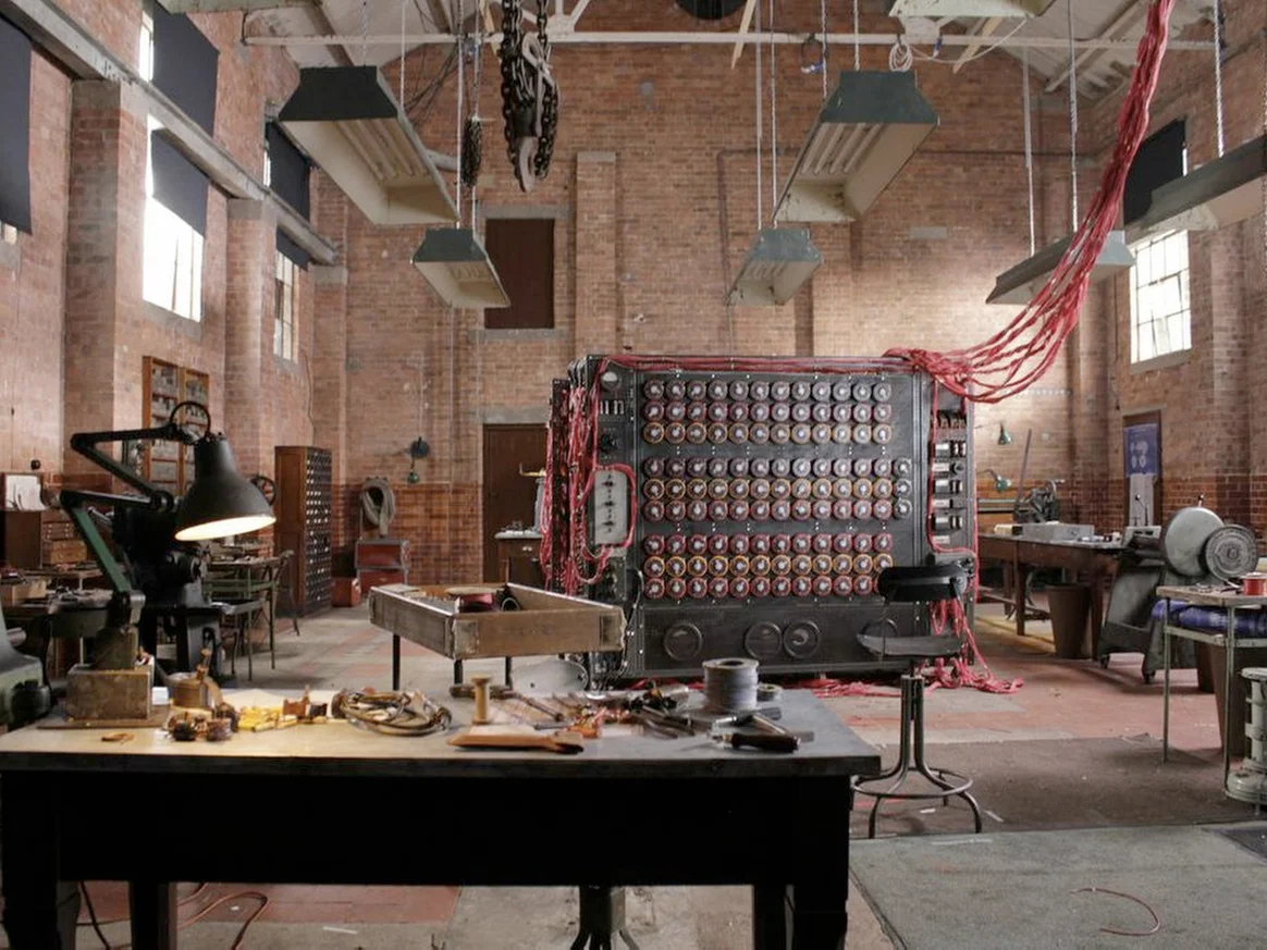
Turing’s early theoretical work was of course useful when he later designed real computers. Turing developed some of the very first computing devices during WW2 to break the Germans’ Enigma codes. If you’re interested in this (and it’s a fascinating story!), I recommend the film The Imitation Game, starring Benedict Cumberbatch as our man Turing.
The film also covers how Turing was persecuted by the government for his homosexuality. In the 1950s, the British government viewed homosexuality as moral degeneracy (which is a bit rich considering what the British state was getting up to in the 1950s) and required Turing to accept female hormones as “treatment”.
Conclusion
Turing is regarded as the founding father of computer science because he developed the first accurate description of what it meant to compute. In his paper, he described a very simple device that could read and write symbols on a tape. Turing argued that this device was capable of computing anything computable and proved that there is no more powerful model.
All of this is very impressive and Turing is only getting started! In the rest of his paper he presents the halting problem and its implications for the original question of automatically deriving theorems. We’ll cover the halting problem in detail in a later article.
Credits
[1] by NACA (NASA) - Dryden Flight Research Center Photo Collection - http://www.dfrc.nasa.gov/Gallery/Photo/Places/HTML/E49-54.html, Public Domain, https://commons.wikimedia.org/w/index.php?curid=885426
[2] Still from “The Imitation Game”.
Keep going with The Computer Science Book.
A guided, opinionated walkthrough of the computer science fundamentals behind posts like this one — from computer architecture to algorithms to modern AI. Thirteen chapters, built for self-taught developers.
Buy the ebook - $19.99Ebook includes PDF and EPUB formats and a 28-day money-back guarantee.