Theory of computation

Introduction

We begin our exciting journey through computer science by looking at just what it is computers actually do: computation. The branch of computer science that explores the capabilities and limitations of computation is known as theory of computation or computational theory. It builds and analyses mathematical models to probe computation in the abstract.

I promised lots of practical computer science information in this book. So why are we starting off with all this abstraction? A good craftsman should have a deep understanding of how their tools work. As programmers, we structure computation in order to achieve results. The better we understand what our computers can and can’t do, the better programmers we will be. You don’t want to waste a week trying to solve a problem that’s been proven to be unsolvable! Secondly, the terms and concepts from theory of computation pop up surprisingly often in day-to-day programming and it’s useful to have at least an acquaintance with them.

Finally, theory of computation is where computer science anchors itself to mathematics, logic and philosophy. It provides the foundations for everything else and will help you to develop a much more sophisticated understanding of what computing is and why computers work. It’s super interesting!

Because of the mathematics, theory of computation has a reputation for being very abstract and dense. Certainly it’s very maths heavy and the textbooks contain plenty of proofs. If you’re not mathematically confident, don’t let that hold you back! Lots of important results are straightforward to grasp without any mathematical background.

Theory of computation is made up of three main areas: automata theory, computability theory and complexity theory.

Automata theory is all about using mathematics to create computational models and explore what they can do. The reason for doing this is that physical computers are hugely complex devices that vary wildly in their design and performance. By using mathematical models, we can strip away all of these superfluous details and better understand the capabilities of the underlying model. We’ll see that an surprisingly simple model of computation is capable of representing any computation.

Once we have the necessary mathematical models we can use them to explore the capabilities and limitations of computation itself. This is computability theory. As we’ll see, there are some surprising limits to what can be computed. Besides being a fascinating intersection of computing and philosophy, you’ll regularly hit against these limitations in everyday programming so it’s vital that you’re aware of them.

After those two sections, we’ll be close to having a solid theoretical base. We’ll still need to sort out a few simple concepts: time and space. Complexity theory is the branch of computational theory that investigates the complexity of algorithms by analysing the resources, primarily time and space, that they require. It gives us ways to understand and measure algorithmic performance and how to classify algorithms according to their complexity.

Automata theory

Let’s begin by asking ourselves: what do we actually mean by the words “computation” and “computer”?

In mathematics we don’t really care how results are worked out. I can assign the square root of a number to a variable and blithely use that variable in equations without worrying about how to actually calculate the square root. My calculator doesn’t have it so easy. It has to know some sequence of steps that will calculate the square root so that it can show me the result. My calculator is performing computation.

A computer, then, is any machine that performs a computation by executing a defined sequence of operations, known as an algorithm. It may optionally generate some kind of result at the end. The particular state of the machine at any given moment indicates the state of the computation. This is a really important concept. A computer is something that takes a list of operations and converts them into some kind of observable form. In my trippier moments I like to imagine that a computer takes a verb (the instruction) and converts it into an object (the state) that represents the outcome of that instruction. The next instruction is then executed against the object, generating a new object that forms the input for the next instruction and so on. Far out!

Note that nothing in this definition requires the computer to be an actual, physical device. We could represent a computer by drawing on paper some states and arrows specifying rules for moving between them. We’ll see diagrams like this below. When defined with a more robust mathematical notation these models are known as automata, from the Greek automatos meaning “self-acting”.

Automata theory determines the capabilities and limitations of various automata designs. In our exploration of the subject we’ll start with the most basic model: the finite automaton. We’ll see that it can do a surprising amount but is ultimately limited by its simple design. We’ll then see how to amend its design to create the more powerful push-down automaton. Finally, we’ll look at the most powerful automaton of all: the Turing machine.

The point of all this is not to come up with a blueprint for a real computer. The point is to find a mathematical model that is both simple to understand yet powerful enough to model any arbitrary computation. Spoiler: such a thing exists and is the Turing machine. Once we have a model for performing arbitrary computation, we can analyse that model to better understand computation itself. Our aim here is to put together the necessary tools so that we can study computation in the abstract.

Finite automata

We have already defined a computer as a machine that can transition through a series of states, each reflecting a step in some algorithm. If there is only a finite number of states and a finite number of transitions, then such a machine is known as a finite automaton or finite state machine (FSM). The finite automaton is the simplest kind of computational model. It’s very useful for modelling primitive devices.

For example, this state diagram represents a turnstile. You may not have thought of a turnstile as a computer but look carefully and you’ll see that it meets our definition above:

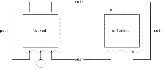
We designate one state to be the start state. This is marked on the diagram by a circle with an arrow pointing to locked. This is the state our turnstile sits in, waiting for something to happen. At each state there are two possible inputs: push and coin. Pushing a locked turnstile doesn’t do anything – it remains locked. We represent this with an arrow looping back to the same state. Inserting a coin causes the turnstile to transition to the unlocked state. Inserting more coins has no effect. As the turnstile is now unlocked, a person can push through, thus resetting the turnstile back to its original locked state.

The possible ways of moving between states are defined by the transition function:

1 transition :: (oldState, input) -> (newState, output?)

I’m using Haskell-like type signature syntax here. The double colons mean “is of type”, so transition is a function that takes a state and an input and outputs a new state and an output. The question mark on output is my way of indicating that it’s optional.

Laying out all of the valid transitions creates a representation of the FSM known as a state transition table:

Even this very simple automaton has a limited form of memory. If the automaton is in the unlocked state we know that the previous input was a coin. But once we transition back to locked we lose this information. We have no way of telling whether a locked turnstile has never been unlocked or whether it’s been unlocked thousands of times.

A machine is deterministic if it consistently gives the same output for a given input. This is generally a desirable quality. An automaton is a deterministic finite automaton (DFA) if there is only ever a single possible transition from each state for a given input. You can see from the state diagram above that the turnstile is deterministic because each input only appears on a single transition at each state.

We can define a non-deterministic finite automaton (NFA) simply by allowing multiple transitions from a state for a given input. This requires a minor change to the transition function:

1 outcome :: (newState, output?)
2 transition :: (oldState, input) -> [outcome1, outcome2...]

For each pair of state and input there may be zero or more transitions. Each transition outputs a new state and optional output. On a state machine diagram this is represented simply by having multiple labels on transition arrows. This raises an obvious question: if a NFA has two available transitions for a given input, how does it choose which transition to take?

The surprising answer is that the NFA follows every possible transition. Remember that we’re talking about mathematical models here. Each time it is faced with multiple transitions, the NFA duplicates itself and each duplicate follows a different transition. Duplicates can in turn duplicate themselves whenever they encounter more transitions. The NFA works a bit like the broomstick from the Sorcerer’s Apprentice, duplicating and reduplicating itself as necessary to cover every possible path.

The duplicates all run in parallel, each one following a different computational path. If one of the duplicates reaches a state where it has no more open transitions, then it’s stuck in a dead end and can be removed. We’ll end up with a whole herd of automata, representing the complete set of possible paths through the transitions. If one of them reaches an accept state, the path it represents is a valid path. We say that the automaton has accepted the input if there is at least one valid path.

This definition applies to deterministic automata too. A DFA is a NFA that just happens to only ever have one possible transition for a given input. This means that a DFA is also a valid NFA. What’s more, any NFA can be represented as a valid DFA. In fact, deterministic and non-deterministic automata are equivalent. Anything that can be computed with a DFA can be computed with an NFA and vice versa. Given this, it seems that NFAs add quite a lot of complexity for a questionable advantage. Why bother? The benefit is that some computations can be more concisely expressed (using fewer states) as a non-deterministic automaton than as a deterministic automaton.

Finite automata, whether deterministic or non-deterministic, are very simple beasts. In fact, they’re so basic that you might at first not even recognise what they’re doing as computation. It appears that finite automata are nothing more than a starting point on our journey. Yet they have another trick up their sleeve. Finite automata pop up surprisingly often embedded in other programs. I’ll refer to code versions of finite automata as state machines. They will appear in codebases you work on, either explicitly or implicitly defined. They’re super useful for modelling processes that flow through a series of states. When you recognise that you’ve got an implicit state machine lurking in your code, pulling it out into an explicit structure can be a great way to manage complexity. This is called the state machine pattern.

Take a complex, multiple step user flow. A good example would be Airbnb’s identify verification flow. Each step in the flow can be represented by a state in a state machine. The actions in the flow are the transitions between states. You might have a state in which you ask the user for basic contact information. When they input their details, the state machine transitions to another state in which the user is asked to upload a photo of their identity card. The upload triggers another transition to a state in which the photo is sent to an analysis service that compares the identity card’s details to the information provided by the user in the first state. If everything matches, the state machine transitions to a success state. If there’s a problem, the state machine transitions to an error-handling state. The user is informed and given the option to repeat the upload process.

It’s possible to do all of the state management and validation manually but it’s brittle and error-prone. Let’s see how the above flow might be implemented without a state machine and then see whether a state machine improves things:

 1 class User
 2   enum status: [:new, :info_provided, :pending, :verified, :rejected]
 3 end
 4 
 5 class UserSignupFlow
 6   def new(user)
 7     @user = user
 8   end
 9 
10   def perform
11     if !@user.status == :info_provided
12       @user.contact_info = get_contact_info
13       @user.status = :info_provided
14     end
15 
16     if !(@user.status == :pending || @user.status == :verified)
17       @user.photo = get_id_photo
18       @user.status = :pending
19     end
20 
21     if IDValidator.valid?(photo, contact_info)
22       @user.status = :verified
23     else
24       @user.status = :rejected
25     end
26   end
27 end

That looks like a mess and I haven’t even handled retrying the photo upload. Admittedly, the code could be tidied up a little by extracting things out into methods and so on. Either way, you can’t get around the fact that perform has to check the status attribute of the user to determine if an action is permitted. In a small flow this is probably manageable, especially with good unit testing. However, it will be very easy to cause subtle errors by performing an incorrect check. This will lead to the user incorrectly transitioning to an invalid state that might not manifest itself until much later in the program. The transitions are not explicitly defined and instead have to be inferred from the conditional clauses, which can easily be incorrectly modified. This is a design that will not scale well at all.

The use of the status attribute is a sure sign that we have an implicit state machine on our hands. Let’s make it explicit:

 1 class UserSignupFlow
 2   include AASM
 3 
 4   aasm do
 5     state :new, initial: true
 6     state :info_provided
 7     state :pending
 8     state :verified
 9     state :rejected
10 
11     event :get_info
12       transitions from: :new,
13                   to: :info_provided,
14                   before: :get_contact_info
15     end
16     event :get_photo
17       transitions from: [:info_provided, :rejected],
18                   to: :pending,
19                   before: :get_id_photo
20     end
21     event :validate
22       transitions from: :pending, to: :verified do
23         guard do
24           IDValidator.valid?(photo, contact_info)
25         end
26       end
27       transitions from: :pending,
28                   to: :rejected,
29                   after: :notify_user
30     end
31   end
32 end

Here UserSignupFlow is re-implemented using the AASM gem in Ruby. Other implementations are available and will vary syntactically somewhat but the fundamentals should remain the same. AASM is neat because it provides callbacks (before, guard, after etc.) that allow you to schedule behaviour around transitions. AASM will also raise an error if we attempt to perform an event on invalid state. Such features give us reassurance that, for example, the user will never end up verified without first having their photo and contact information validated. In a real world application it would be trivial to refactor this by adding more states and transitions, creating more complex events and so on. Things are much easier to reason about because we explicitly model the possible states and valid transitions between them.

Regular expressions

There is one other hugely important use of finite state machines that I haven’t touched on yet: regular expressions (regexes).

Recall that a finite automaton can define accept states. If an input causes the automaton to finish on an accept state, then the input is accepted. Another way of phrasing this is to say that the automaton recognises the input. This is exactly what regular expressions do! Whenever you write a regex you are actually using very terse syntax to define a tiny finite state machine that will recognise, or match, particular strings.

Take the regex (a|b)+c. We can express this as a NFA that accepts at least one a or b and then a single c. The double border identifies the accept state:

We refer to the set of valid inputs (e.g. ac, bc, abac) as the language of the automaton. Languages that can be recognised by finite state machines are called regular languages, from which we get the term “regular expression”.

Many theory of computation textbooks define automata in terms of what languages they can recognise. Languages and their automatons are more or less equivalent – one can be defined in terms of the other. The more complex the automaton, the more sophisticated the class of languages it can recognise. For now, it suffices to know that finite automata can only recognise regular languages. They are at the bottom of the hierarchy.

I think it’s pretty cool that we’ve only looked at the simplest automaton and we can already understand how regexes are constructed. Next time you write a regex, try and work out how it could be expressed as a finite automaton. Sadly, this neat pedagogical picture is complicated by reality. Many modern regex engines include features (e.g. back referencing) that allow them to accept non-regular languages. Why would they need to do this? Though finite automata are surprisingly capable little creatures, their simple structure does impose sometimes significant limitations.

For instance, we cannot create a regular expression (i.e. define a finite state machine) that tells us whether a given string has a balanced number of parentheses. What we want is an automaton that accepts an input like ((()())) but rejects (())). It’s easy to sketch out a state machine that can recognise our example input (try it yourself) but we cannot create a finite automaton that accepts every valid input. The problem is that the number of parentheses is potentially infinite, meaning that we’d need to have an infinite number of states. This is obviously incompatible with it being a finite automaton. We need some way for the automaton to “remember” what it has seen before without having to encode it as a state.

Push-down automata

As we saw previously, a finite automaton has no memory beyond its current state. To recognise matching parentheses we need some kind of scratch space where the automaton can keep track of how many parentheses it has seen so far. This requires a new, more complex model of computation known as a push-down automaton:

A push-down automaton is a finite automaton combined with a stack: a last-in, first-out data structure. Think of a stack of trays in a cafeteria. Clean trays get put on top of the older ones and the next customer to come along will take a tray from the top. The last tray to be added is the first to be taken. We can interact with the stack via two operations. We can push a value on to the top of the stack. We can also pop, or remove, the newest value off the stack. Doing so exposes the second-newest value as the new top. The number of items that can be pushed on to the automaton’s stack is infinite. The set of values that can be written to the stack is called the stack alphabet. We need to start the stack off with an initial value from this alphabet.

We must update the transition function to enable access to the stack. We can read the value on the top of the stack and optionally perform an operation on the stack:

1 stackOperation :: Pop | Push
2 transition :: (state, input, topOfStack) -> (state, stackOperation)

Equipped with this new functionality we can make short work of checking for balanced parentheses. Every time the input is a ( we push a ( on to the stack. Whenever we come to a ), we check that the top of the stack is a ( and pop it off. If we encounter a ) or an empty stack, then we know that the parentheses are unbalanced. If we get to the end of the input and have an empty stack, then we move to an accept state and recognise the input as valid.

In the diagram above, the input is recorded as symbols on the tape along the bottom of the diagram. The tape is read from left to right. The stack that the finite automaton can manipulate is on the right. Note that the values of the stack alphabet don’t have to match the input alphabet. They happen to do so in this case but it’s not required. The diagram shows a computation in progress and so there are a couple of parentheses already on the stack. Will this particular example end up in an accept state? Well, so far we can see two ( have already been pushed and there is another about to be read from the input tape. After that we can see three ). Assuming that the input ends after these three values, the automaton will pop three ( off the stack, leaving an empty stack at the end of input. The input is valid.

The stack is a very simple data structure but it gives the automaton an unlimited amount of memory to work with. We can use this to keep track of what the automaton has already seen without requiring explicit states for each possible input. This is from where the push-down automaton derives its additional computational power.

Turing machines

Though useful, a stack is still limited in its own way. We can only ever read the top-most value. When we want to get at a value further down the stack we need to pop off all of the values on top. This entails discarding the values since we have nowhere else to store them. What we would really like is a way to read or write to any location in memory. We need a more complex automaton.

In 1936, before any physical computer had ever been built, the mathematician Alan Turing published a paper describing an automaton that meets our requirements. It consists of a finite automaton “control unit” that reads instruction symbols from an infinitely long tape, just like our push-down automaton above. The two crucial differences are that the tape head can move left as well as right and that it can write values as well as read them. Turing called this automaton an “a-machine” (for “automatic machine”). Nowadays it is more commonly known as the Turing machine in his honour.

The machine starts with the tape head at the beginning of the instruction sequence. The rest of the tape is blank. At each step of the computation the machine reads the current value under the tape head, updates the current state, writes a value to the current tape position and then moves a single step to the left or right. The transition function therefore looks like this:

1 shiftDirection :: Left | Right
2 transition :: (state, tapeValue) -> (state, newTapeValue, shiftDirection)

Note that newTapeValue might be identical to tapeValue, resulting in no change to the tape. We say that the machine halts if it eventually moves into an accept or reject state. If it doesn’t halt, it will loop indefinitely.

What can we do with these Turing machines? On the surface it seems simpler than the push-down automaton because it does away with the separate stack. In fact, having read/write access to any arbitrary location on the tape makes the Turing machine much more powerful. One of Turing’s great achievements was to prove that the Turing machine is the most powerful automaton possible. If a solution to a problem can’t be computed on a Turing machine, there is simply nothing else that might be able to compute it. Therefore, we can actually use Turing machines to define computation. A problem is computable only if it can be solved on a Turing machine. This is known as the Church-Turing thesis after Alonzo Church and Turing, who both independently found the same results (see the further reading for more on Alonzo Church). The implication of the thesis is that every computable problem has a corresponding Turing machine. Discoveries like this are why automata theory is worth studying. It gives us direct insight into the nature of computation itself.

Yet how was Turing so sure that there is nothing more powerful than his machine? Recall that the transition function takes the current state and tape value and outputs a new state, new tape value and shift direction. As with a finite automaton, the transition functions for each state and tape value pair form a state table that defines the machine’s operation. If we wanted to change how the machine operated, we would need to change the transition functions. We can’t because these are hard coded into the structure of the finite automaton control unit. Changing this would effectively create an entirely new machine.

There’s a better way. Turing demonstrated that it is possible to encode the structure of the control unit as a string. That means that it can be written on the input tape. We can therefore encode a “virtual” Turing machine on to the tape along with the instruction symbols. This tape can be read by a second, “real” Turing machine with a control unit designed to decode and emulate the virtual Turing machine. The real Turing machine shuttles back and forth between the instruction symbols and the virtual Turing machine definition, executing the instructions just as the virtual machine would have done. What we end up with is a Turing machine that emulates the behaviour of the virtual one:

1 Host(Virtual, input) accepts if Virtual(input) accepts
2 Host(Virtual, input) rejects if Virtual(input) rejects
3 Host(Virtual, input) loops if Virtual(input) loops

Such a Turing machine is known as a universal Turing machine. Thanks to the Church-Turing thesis, we know that every computable problem has a Turing machine. A machine that can emulate any Turing machine can therefore emulate a Turing machine solving any computable problem, which is the same as actually solving it. Therefore any computable problem can be solved by a universal Turing machine.

Bear in mind here that we’re talking about the capabilities of mathematical models. It’s certainly possible to create a physical computer that can perform faster or more efficiently than some other computer. In this sense computers have become vastly more powerful. But there is nothing that a modern computer can compute that a Turing machine can’t also compute, given enough time. This might seem surprising but it also makes intuitive sense. When you upgrade your computer’s processor you don’t suddenly gain access to a whole new class of computation that was previous inaccessible. You can simply do the same computation in less time. This performance improvement might be enough to enable new functionality – perhaps moving from rendering 2D graphics to 3D – but this is solely because the time taken by the slower processor was deemed unacceptable by the user.

Is a real computer a Turing machine? After all, they look a little similar. If you squint a bit, the tape head capable of reading and writing at any point on the tape is a bit like a processor reading and writing at arbitrary memory locations. A Turing machine, being a mathematical concept, is able to use an infinitely long tape. Real computers, however, have to make do with a limited (though nowadays very large) amount of memory. Something that is computable on a Turing machine may therefore not be computable on a particular physical computer without running out of memory.

Remember that a Turing machine is not meant to be a simple blueprint for a computer. It’s a simple model of computation that is powerful enough to model any arbitrary computation. We can now explore the capabilities of the Turing machine in order to determine the properties of computation itself.

Computability

Computability theory is the second of the three branches of theory of computation. It asks things like: what is a computable problem? Are there problems that can’t be computed? Thanks to our exploration of automata theory, we can approach these questions with the assistance of the Turing machine.

What is a computable problem?

As we saw above, there is no computational model more powerful than the Turing machine. Therefore, a problem is computable if it can be solved on a Turing machine. The execution steps performed by the Turing machine form an algorithm and so we can also define “algorithm” in terms of a Turing machine: an algorithm is anything that can be executed on a Turing machine. It is not possible to have an algorithm that can’t run on a Turing machine.

We saw above that Turing created the universal Turing machine: a Turing machine that can simulate another Turing machine. If a computational method is capable of simulating a Turing machine, and therefore performing any computation, we say that it is Turing complete. One Turing complete computational method is as powerful as another. Usually Turing completeness is what you want. If you’re writing a general-purpose programming language, then it’s essential that users can write arbitrary computations. The majority of programming languages are therefore Turing complete. Anything you can do with one Turing complete language you can achieve with another. After all, it would be absurd to look at a problem and think “well, this is solvable in Ruby but not in Go”.

Let’s prove that intuition. Suppose that a problem did exist that was solvable in Ruby but not in Go. It’s possible to write a Go program, known as an interpreter (see the compiler and interpreters chapter if this concept is new to you), that takes Ruby source code as input and simulates executing the Ruby code. That means we can just express the problem in Ruby and run the Ruby code through our interpreter written in Go. Therefore the problem is solvable in Go.

In practice, of course, different languages might be better suited to different tasks This doesn’t imply any difference in language capability. It’s merely a question of what’s more ergonomic for the programmer.

Amusingly, things sometimes become Turing complete by accident. Pokémon Yellow is a great example. In a game, every player input triggers some computation that updates the program state. Normally, a game will only allow you to perform limited computation. Moving your character around computes a new position and writes it to memory, acquiring an item updates the inventory and so on. It’s been demonstrated that a bug in Pokémon Yellow allows you to update arbitrary memory locations by performing specific actions. You can basically reprogram the game to do what you want. In the further reading section there’s an example of someone reprogramming Pokémon Yellow to become a music player. Once you have demonstrated Turing completeness, all bets are off!

It’s hard to overstate the importance of Turing’s 1936 paper. In one fell swoop he designed an automaton capable of modelling any computation and demonstrated that other computational models could be equivalently powerful but no more. Unfortunately for the fledgling discipline of computer science, Turing also demonstrated that his machine had some striking limitations.

Are there uncomputable problems?

We know that any computable problem can be solved using a Turing machine. Are there problems that are uncomputable altogether? Some problems with subjective answers self-evidently don’t make sense as a computational problem e.g. “which of these paintings is the more beautiful?”. There are also problems that seem like they should be straightforward but are actually uncomputable:

Do functionA and functionB behave in the same way for all inputs?
Does a given function print “hello, world”?

I use the term “function” here in order to express them as problems that might come up in programming. A function defines an algorithm and an algorithm defines a Turing machine so the three terms are broadly interchangeable.

You might think that the first problem could be easily solved by passing in many different inputs to both functions and checking that they behave in the same way. Such an approach can give us reasonable confidence but we can never be absolutely sure. Since the number of possible inputs is infinite, we can never be sure that the two functions might not behave differently for some as yet untested input.

The second problem is more surprising. Remember that a Turing machine will either halt or continue indefinitely. If it halts then we can just check whether it outputted “hello, world” before halting. The problem occurs when it does not terminate. We can tell that it hasn’t printed “hello, world” yet, but we can never be sure, in every possible case, that it won’t eventually print the string. We need to let it run for a potentially infinite length of time. We can therefore rephrase this problem in more general terms:

Does a given function halt on a given input?

This is known as the halting problem because we can’t know if a Turing machine implementing the computation will ever halt. Let’s look at an example.

You work at some hot new startup that provides lambda functions over blockchain. Your users upload small functions that you execute on a server farm before writing the results out on to a blockchain. Your users are happy because they don’t have to worry about servers and your investors are happy because your startup uses a blockchain!

You, however, are not happy. Some of your users keep writing broken functions that end up in infinite loops, hogging your server resources and requiring you to go in and stop them manually. Your boss, who has an MBA background, asks if you can write a program that will scan users’ uploaded code and check for infinite loops before letting them run on the server farm. How would you go about solving this? You write a static analysis tool that examines the source code without running it and finds obvious loops like this:

1 function f() { g(); }
2 function g() { f(); }

Your analysis tool runs on every uploaded function. It catches many infinite loops but still plenty get past your checks. You’re missing something. Looking at what your users upload, you see that often mutually recursive functions don’t directly call each other, as f and g do. There might be any number of intermediate function calls obscuring the relationship. Sometimes the uploaded code stores functions in data structures and moves them around or even generates them at runtime. No matter how thorough your tool is, static analysis just isn’t going to cut it. You’re going to have to actually run the code to see how it behaves. This raises a new problem. How can you tell the difference between a program caught in an infinite loop and one in a very slow but finite loop? Try as you might, what you will eventually discover is that there is no way to write a program that will tell you in all cases whether a given program will terminate or loop infinitely on a given input. This is the halting problem.

It’s surprisingly easy to write a proof by contradiction of the halting problem in code. If you haven’t come across a proof by contradiction before, the idea is simple. Assume that the thing in question is true. Work through the consequences until you hit a contradiction. Since there’s a contradiction, the thing in question must not be true. Let’s assume that it is possible to write a function that determines whether a given function will terminate (i.e. halt) on a given input:

1 function terminates(program, input) // returns bool

This function signature shows that it takes a function called program and an input and returns a boolean value showing whether or not program returns when given that input. Assuming the existence of this function, we can write an inverse function that does the opposite:

1 function inverse(program, input) {
2   if terminates(program, input) {
3     while(true) { continue; } // loop indefinitely
4   }
5   return // halt
6 }

If program(input) halts, then inverse(program, input) continues indefinitely and vice versa. What happens if we pass inverse to itself?

1 function inverse(inverse, input) {
2   if terminates(inverse, input) {
3     while(true) { continue; } // loop indefinitely
4   }
5   return // halt
6 }

Don’t worry if you find the recursion a bit mind-bending. If terminates(inverse, input) evaluates to true then we loop indefinitely. But that means that terminates(inverse, input) should return false! But if it returns false then inverse will return and so terminates(inverse, input) should return true! It seems that terminates(inverse, input) has to return both true and false at the same time. We have found our contradiction and conclude that terminates does not exist after all.

Expressed in more abstract terms, we have proved that it is impossible to create a Turing machine that takes another Turing machine and determines whether it will loop or halt on a given input. In some respects this is actually quite a reassuring result. For one thing, if it were possible to determine whether a computation would halt, it would have huge implications for mathematics. We’d be able to prove lots of conjectures by showing that a program would eventually halt after finding a counterexample to the conjecture. For example, the Goldbach conjecture states that every even number greater than two is the sum of two prime numbers. Currently it’s unproven. We could write a program that would iterate through every even number greater than two and check whether it’s the sum of two primes. It would run until it finds the first counterexample, at which point it halts by returning the counterexample. If we could solve the halting problem, we could determine whether this program would ever terminate and so prove or disprove the Goldbach conjecture. Such a program would in effect “short circuit” the computation by getting the result without having to do the work to find the counterexample. Intuitively it doesn’t make sense.

Moving back from mathematics, the key take away for a working programmer is to be wary of any task that requires you to know how long a computation will take. You may be able to make a reasonable guess most of the time but you can never have a general solution that works for all cases. There’s a reason why real cloud services just put a basic timeout on their users’ lambda functions: there’s really no better way to detect infinite loops!

The Entscheidungsproblem and the incompleteness theorem

The Entscheidungsproblem, or decision problem, was posed in 1928 by mathematician David Hilbert. His question, expressed in rough terms, was: “is there an algorithm that can prove whether a given logical statement is true?”. Hilbert’s hope was that it would be possible to find a computational means of discovering mathematical theorems (i.e. true mathematical statements). Once written, this program could be left to beaver away and uncover wonderful new theorems.

Kurt Gödel dealt a blow to Hilbert with his first incompleteness theorem, published in 1931. This states that any “sufficiently expressive” formal system for expressing truth will be incomplete, meaning that it will include statements that are true but unprovable by the system’s rules. Turing’s 1936 paper used Turing machines to demonstrate this. His reasoning was that the “algorithm” to solve the decision problem could be expressed by asking whether the algorithm’s corresponding Turing machine would halt. Since there was no general solution to the halting problem, there could be no general solution to the decision problem.

If every true statement can be proved, then we could write a program that took a statement and generates candidate proofs until it halted on one that either proved or disproved the statement. Since the number of possible proofs is infinite, we are back to asking whether a Turing machine will halt or loop indefinitely. It appears that there are some problems, such as the Entscheidungsproblem and the halting problem, for which it is simply impossible to write an algorithm that will always give the correct answer. Such problems are undecidable.

Is it just me or are things getting pretty heavy? Let’s look at a concrete example.

After the great Bitcoin crash, your investors lost interest in your lambda function blockchain startup. You find a new job building a digital catalogue system for a library. At least here you should be safe from impossible tasks! Your first job is to create a catalogue of every resource in each section of the library: cars, computing, fiction etc. This is straightforward. Flushed with success, you next create an overall catalogue of every resource in the entire library. Just as you’re finishing, you realise that the section catalogues need to be included in the overall catalogue too. In fact, the overall catalogue is itself a library resource and so should be included in itself. Clever!

Your boss is pleased by your industriousness but is getting confused by the profusion of catalogues on the system. She asks you to create a catalogue of all the catalogues. Easy! On showing it to your boss you remark that you’d remembered that the catalogue of all the catalogues should include itself since it’s a catalogue too. This is all a bit too much for your boss and she tells you that she’d much rather have a catalogue of just the catalogues that don’t include themselves. When you put this together you run into a problem: should this catalogue include itself? If it doesn’t include itself then it will be an example of a catalogue that doesn’t include itself and you would be remiss in leaving it out. Yet if you do add it in, the catalogue will include itself and so won’t meet the requirements for inclusion. Whatever you do will be wrong!

Does this remind you of the proof by contradiction of the halting problem? An even simpler example is the liar’s paradox: “this sentence is false”. Its simplicity makes the root of the problem obvious: the statement is self-referential and leads to paradox. When you follow the logic of either the catalogue example or the liar’s paradox, you find yourself caught in an infinite loop: it is false, therefore it is true, therefore it is false, therefore it is true and so on. The infinite loop means that we cannot prove the statement to be either true or false. Because the algorithm loops infinitely, a corresponding Turing machine will also never halt.

Gödel’s work is complex and requires a sophisticated understanding of logic to really comprehend deeply. My explanation is by necessity very high level, but I hope that these analogies give you some glimpse of the incompleteness theorem’s implications. It is perhaps easier to understand in terms of its connections to other fields. Finding a solution to the halting problem, for example, would imply that a solution to all the above paradoxes existed. The behaviour of the Turing machine gives an intuitive, mechanical expression to Gödel’s profound insights.

Algorithmic complexity

We have a better understanding of what computation is and isn’t. Next, we consider how computation behaves. How does one algorithm compare to another? A very important metric is the algorithm’s complexity. We measure the complexity of an algorithm in terms of how many resources it needs. The two most important resources in a computer are the amount of processing time something needs and the amount of space in memory it consumes. Usually the resource usage depends on the size of the input so we’d like to know how these requirements change as the input changes.

The time an algorithm takes to complete is known as the running time. It’s commonly measured by how many steps the algorithm takes or by how long a computer spends executing the algorithm. Obviously the exact running time will vary from machine to machine but what we’re most interested in is the relationship between the input size and running time. By “size” we technically mean how many symbols a Turing machine needs to encode the input, but it’s easier to think of it as literally referring to the length of a string input. Let’s say we have an algorithm that takes a certain amount of time to execute for an input of length n. If the input length increases to n + 1 will the algorithm use the same time, a little bit longer, twice as long or maybe even longer? Failing to consider this could lead you to write code that works wonderfully on small, test inputs but falls over as soon as it has to handle large inputs. That is undesirable.

Turning to space requirements, an algorithm might require a large working space to hold intermediate values or generate data structures. On a Turing machine this is no concern because the tape is infinitely long. Real computers don’t have this luxury and must make do with a finite amount of memory. Does the computer have sufficient memory to contain the working space required by the algorithm? Will it run out of memory if we give the algorithm a larger input?

Nowadays computers have absurd amounts of memory and so space is generally less of a concern than time. It’s fairly common, as I will do, to focus on the running time of an algorithm as the key measure of performance. Bear in mind that the exact same principles apply to measuring space requirements. This can still be a major problem on memory-constrained mobile devices.

It’s often possible to improve an algorithm’s efficiency to use less space or take less time. But as the computing gods give with one hand, they take with another. There is usually a trade-off between optimising for time and for space. For example, in some cases it’s possible to reduce running time by using a technique called memoisation to cache intermediate values and avoid recomputing them at a later step in the algorithm. The time saved comes at the cost of using more space to store those intermediate results.

We want to describe how the time and space requirements of an algorithm change as the input size changes. We need a way of expressing this that’s both simple and makes it easy to compare algorithms. Computer scientists have developed a pleasingly rough form of estimation called big-O notation. The basic observation behind big-O notation is that we can model the running time of an algorithm as a ratio of the input size to the running time. The ratios of simple algorithms can be combined to describe the behaviour of more complex ones. Let’s take two hypothetical functions:

As the names suggest, the running time of double is always double the input size and square’s is the square of the input size. Now let’s look at another function that first performs double and adds it to the result of square. Its running time would therefore be the sum of both running times:

Let’s see how the running times of double and square change as the input size increases:

As you can see, the running time of square increases at a much faster rate than that of double. This means that as the input size grows, the contribution double makes to the total running time of squareDouble becomes smaller and smaller. For really large inputs it’s insignificant. The key idea behind big-O notation is that we can get a rough idea of an algorithm’s complexity just by looking at the ratio of its most significant component. That’s the bit that makes the biggest contribution to the algorithm’s running time. In the case of squareDouble, it’s square. Even if we have a big, complicated algorithm with lots of bits contributing to the total running time, we can just ignore everything except the element that makes the biggest difference to the running time.

We can simplify even further. What if we had a function called triple that had a time requirement of three times the input size? Well, it has a ratio of 3n, which is clearly bigger than double’s 2n, but as the input size increases, they both quickly pale into insignificance compared to square’s n2. In a wonderful flourish of contempt, big-O notation declares that the coefficient, the number in front of the n, is too insignificant to bother worrying about. We focus solely on the ratio. Here’s how we can express the running time of our four functions using big-O notation:

We don’t care that triple is actually slightly slower than double because, for very large inputs, they perform roughly the same as each other in comparison to square. Similarly, squareDouble is slightly slower than square, because of the additional 2n in its running time, but the difference becomes negligible for large inputs.

When using big-O notation, we are only talking about the worst-case performance. The time it takes to iterate through an array to find a value will depend on where in the array the value is located. If the value is at the very beginning of the array, it’ll take less time than if it’s at the very end. Being pessimists, we always assume the worst case. Big-O notation shows us the upper bound on the algorithm’s requirements – at least it can’t get any worse!

There are two main ways to determine the complexity of an algorithm. The first is to simply look at the code and see how it behaves. This works for simple cases written in relatively low level languages, such as C, where the structure of the code closely matches the operation of the algorithm (hence the popularity of teaching algorithms in C). In higher-level languages, such as JavaScript or Ruby, a lot of computational steps can be hidden behind function or method calls, not to mention the behaviour of the underlying interpreter. Often the easiest thing to do is just benchmark the running time for various inputs and see what ratio emerges.

We can categorise algorithms by their input size : running time ratio. The most common categories are graphed below:

The flatter the curve, the better. The best is O(1) because it’s a completely flat line and so doesn’t change at all. Some lines, such as O(log(n)), increase very slowly. This is great because it means that an increase in input size doesn’t have too much impact on the running time. Others, such as O(2n), increase almost vertically! This is very bad because even a tiny change in input size has a huge impact on the running time. Look carefully and you’ll see that some curves start off quite slowly and only increase steeply later. There’s a jumbled point in the bottom left where curves cross each other, meaning that one ratio is better up to a certain point and then another is better after that. An algorithm with a “bad” ratio might actually perform well in practice for small inputs. In theory, though, we’re only interested in what happens with really big inputs.

Let’s look at an example algorithm for each ratio. I’m using a C-like pseudo-code so that every step in the algorithm is clear.

Constant O(1):

Constant algorithms, as we’ve just seen, have the same running time no matter the input size. Capitalising the first character of a string is an example of a constant time algorithm. It never has to go past the first character and so the input size has no effect on the running time.

1 string capitaliseInitial(string input) {
2   input[0] = toUpperCase(input[0]);
3   return input;
4 }

Constant algorithms are fairly uncommon, unfortunately.

Logarithmic O(log(n)):

If each increase in input size adds a decreasing amount to the running time, then we have logarithmic complexity. In the chart you can see that the line gradually becomes flatter. In fact, the increase in running time trends towards zero. The cool thing about this is that very large inputs barely require any more resources than smaller ones.

One of the most famous examples of a logarithmic algorithm is binary search (see the algorithms chapter for more details). Below is an implementation that looks for a key in an array of inputs. If it finds the key, it returns the key’s index.

 1 int binarySearch(int[] inputs, int low, int high, int key) {
 2   int middle = (low + high) / 2;
 3 
 4   if (key == inputs[middle]) {
 5     return middle;
 6   }
 7   if (key < inputs[middle]) {
 8     return binarySearch(inputs, low, middle - 1, key);
 9   }
10   if (key > inputs[middle]) {
11     return binarySearch(inputs, middle + 1, high, key);
12   }
13   return -1 // not found
14 }

Observe that each recursive call to binarySearch discards one half of the input. At first low and high cover the whole array, then half, then a quarter, then an eighth and so on. This is a classic indication of a logarithmic algorithm. Sadly, algorithms with logarithmic performance are also fairly uncommon.

Linear O(n):

The resource requirements of linear algorithms increase in proportion to the input size. Each increase in input size adds the same amount to the running time, as you can see by the straight line in the chart above.

Strings in C are terminated with the null character \0. To find the length of a string you iterate through the string until you find the null character:

1 int stringLength(string input) {
2   int i = 0;
3   while (input[i] != '\0') {
4     i++;
5   }
6   return i;
7 }

Each additional character in the input string adds one extra iteration to the while loop and so the algorithm is linear. Such algorithms are very common, particularly for basic operations on collections of values. For more complex problems a solution with O(nlog(n)) running time – a combination of linear and logarithmic – is generally seen as pretty good.

Polynomial O(nx):

An algorithm’s performance is polynomial if an increase in the input size causes the running time to increase by multiples of the entire input size. Often this happens because the algorithm contains nested loops. The running time increases at a much faster than linear rate. The exact rate depends on the value of x. n3 increases more rapidly than n2.

1 printPairs(string letters, int length) {
2   for (int i = 0; i < length; i++) {
3     for (int j = 0; j < length; j++) {
4       print(letters[i], letters[j]);
5     }
6   }
7 }

This algorithm prints every possible pair of characters from a string. The nested iteration is a giveaway that we’re dealing with polynomial complexity. Rather than making a single pass through the input (as we would if the algorithm were linear), we make a pass through the entire input once for every value in the input. In total we make n * n (i.e. n2) iterations, so the performance is quadratic. If there were another nested loop we’d have n3 or cubic performance.

Polynomial performance is bearable but generally undesirable. Nested loops indicate places where a more efficient solution may be possible but they are not always as obvious as the example above. For example, the following code has a performance flaw that is a common gotcha in C code:

1 string capitalise(string input) {
2   for (int i = 0; i < stringLength(input); i++) {
3     string[i] = toUpperCase(string[i]);
4   }
5 }

Do you see the problem? What performance does this function have? On the surface it looks to be linear because there’s only one loop and we know that toUpperCase has constant performance. However, the condition check within the for loop makes a call to stringLength once for each element in the input. Since stringLength performs its own iteration through the input, we end up looping through the whole input once for every input element: quadratic performance!

Exponential O(xn):

The resource consumption of an exponential algorithm grows more quickly than any polynomial. An algorithm with 2n complexity will double its running time if the input increases by just one!

1 int fibonacci(int num) {
2     if (num <= 1) {
3       return num;
4     }
5     return fibonacci(num - 2) + fibonacci(num - 1);
6 }

This inefficient implementation of the Fibonacci sequence has exponential running time because it doubles the number of steps every time n increases by one. Try writing out the steps it performs for n = 3 and n = 4 if you don’t see this. Exponential algorithms often use a brute-force search to solve the problem by trying every possible solution. This is usually impractical for anything but small inputs.

Factorial O(n!):

If you’re not familiar with factorials, 4! is equivalent to 4 * 3 * 2 * 1 and 5! is equivalent to 5 * 4 * 3 * 2 * 1. Each increase in the input size multiplies the running time by n. Factorial algorithms very quickly lead to huge resource requirements and are rarely useful beyond a very small input size. An example of a factorial algorithm is printing every possible permutation of a list.

Looking at the big-O notation again, we can see that constant time and linear time are actually both examples of polynomial time (O(nx)). Constant time is a special case where x is 0 and linear time is a special case where x is 1. You may have noticed that we crossed a boundary when we went from polynomial to exponential. A problem is tractable if it has a solution in polynomial time. This means that the algorithm is efficient enough to be useful, albeit maybe somewhat slow. A problem is considered intractable if it doesn’t have a polynomial time solution. There might be some exponential or factorial solution but it will be so inefficient as to be unusable in practice.

For example, cubic algorithms (O(n3)) are pretty slow and you’d want to avoid using them where you can. But look how the running time compares to an exponential algorithm (O(2n)):

You wouldn’t want a cubic algorithm sitting in a server’s request handler but it’s still unimaginably more efficient than an exponential algorithm.

Complexity classes

A complexity class is a group of problems that all require similar computational resources. They therefore have roughly the same level of complexity. To better understand this we need to introduce a couple of new concepts.

Problem A can be reduced to problem B if you can easily write a solution to problem A by using a solution to problem B. For example, finding the smallest value in an array can be solved by first sorting the array in ascending order and then taking its first element. Once you’ve got the array sorted, taking the first element is trivially easy. The problem of finding the smallest value is reduced to the problem of sorting the array. Because finding the first element is a constant time operation, as we saw above, we say that the problem reduces in constant time.

1 function smallest(values) {
2   return sort(values)[0];
3 }

You might be thinking that this makes no sense! Sorting the array will take longer than just iterating through it once, keeping track of the lowest value seen so far. How can you reduce problem A to problem B if the solution to B is less efficient? At the risk of more theoretical hand-waviness, we treat the solution to problem B as an imaginary oracle that provides the correct answer straight away (i.e. in constant time). Bear with me on this. Just imagine that sort in the example above returns immediately.

Moving on, some problems are known as decision problems. They only provide true/false answers. The problem “is this a valid path between these two points?” is a decision problem. It only asks whether the given solution is valid. The corresponding search problem asks: “which is the fastest path between these two points?”. You can see that the decision problem is easier to solve than the search problem. Answering a search question requires generating a valid solution or demonstrating that none exists.

Armed with these new terms we can begin to explore complexity classes. Problems are categorised in different classes based on the complexity of generating and verifying solutions.

All problems in the polynomial (P) class have a polynomial time solution. These are the tractable problems for which we have efficient solutions.

A problem is in the non-deterministic polynomial (NP) class if a possible solution can be verified in polynomial time. This says nothing about whether an actual solution can be generated in polynomial time. If someone comes to you claiming to have solved a Sudoku puzzle, you can easily verify their solution in polynomial time by checking that no row, column or square has duplicated digits. Actually coming up with a correct solution is a substantially more difficult task.

It appears that this definition bears no relation to the name. Why “non-deterministic”? An alternative definition for NP involves non-deterministic Turing machines that generate guesses for solutions and then verify them. This definition has fallen somewhat out of use, probably because it’s harder to understand, but the name has stuck. Let’s just accept it for what it is and roll with it.

It is self-evident that all P problems must also be in NP. If I give you a claimed solution to a P problem you can verify it in polynomial time simply by rerunning my computation and checking you get the same answer. By the definition of P, this verification can be done in polynomial time. Therefore the problem is in both P and NP.

Is it true that every problem with efficiently verifiable solutions has an efficient algorithm to generate solutions? Every problem in P is in NP but is every problem in NP in P? This is known as the P = NP? problem. It’s hugely important but as yet unanswered. In fact, it’s the biggest unsolved problem in computer science. Theorists generally suspect, but do not know for sure, that P != NP. A great deal of effort has gone into finding efficient solutions to certain NP problems with no success. On the other hand, efficient solutions have been found for some NP problems and no-one has managed to actually prove that P != NP. The question remains open.

The whole issue might seen rather arcane but the implications of proving P = NP would be huge. It would prove that efficient solutions definitely exist for any problem that can be efficiently verified. Public-key cryptography, which is used to encrypt much of the communication on the Internet, relies on P != NP. It’s based on the assumption that brute-force guessing the correct key to decrypt a message is too computationally expensive to be feasible. If it were true that P = NP, this would imply that an efficient key search algorithm exists. Although, if you worked at a three letter agency and found a proof that P = NP that enabled you to decrypt much of the world’s encrypted communications, would you tell the world?

Taking off my tinfoil hat, let’s move on to NP-hard problems. They are, well, hard. They are at least as hard as the hardest problems in NP. A problem is NP-hard if every problem in NP can be reduced to it in polynomial time. A consequence of this is that a solution to one NP-hard problem would allow all NP problems to be solved in polynomial time. As things stand, there is no known efficient solution to any NP-hard problem. To better understand how a single NP-hard problem can be used to solve all NP problems, let’s turn to our old friend: the halting problem. Any NP problem can be expressed as a Turing machine that halts when it finds a valid solution to the problem. It can be reduced to the halting problem simply by asking whether that Turing machine will ever halt. The halting problem is therefore an NP-hard decision problem.

An interesting class of problems are NP-hard but are efficiently verifiable so they are in NP too. Such problems are known as NP-complete. Often the decision version of an NP-hard problem is NP-complete. The most famous example is probably the travelling salesman problem: what is the shortest possible route that goes through a set of cities and returns to the start? Coming up with a solution is an NP-hard problem. But checking whether a proposed route is indeed the shortest is an NP-complete problem. Solving a Sudoku puzzle is another example of an NP-hard problem with a polynomial verification.

Is the halting problem also in NP? Well, it is indeed a decision problem but we can’t verify a solution to the halting problem in polynomial time because the halting problem can’t give us a solution at all. It is undecidable.

Here are the various complexity classes represented as a Venn diagram (assuming that P != NP). You can see how NP-complete represents the overlap between NP and NP-hard:

I promised less theoretical hand-waving and here I am talking about polynomial complexity and magic oracles. Stick with me – this stuff really is useful. You need to know about it because many problems are NP-complete. This means that no-one has been able to find an efficient solution to them. Without meaning to be a downer, it’s unlikely that you’ll suddenly come up with one yourself, so you need to be able to recognise when a particular task is an instance of an NP-complete problem. Unfortunately, many of them have quite obtuse names like the “subset sum problem” or the “subgraph isomorphism problem”. In the further reading is a link to Karp’s 21 NP-Complete problems, which provides an overview of common problems.

To give some concrete examples, maybe you were fired from the library after the whole catalogue incident but have been taken on at a new Uber-for-bikes startup. Given a list of people who want to be picked up at specific locations and times, how best do you allocate all of the available bikes? This is an NP-complete problem. How do you arrange the seating plan at a wedding so that people sit with people they like and not next to people they dislike? This is NP-complete. If you have a list of backup files of varying sizes and a set of disks with varying amounts of free space, how do you fit all of the backups on the disks? Again, NP-complete.

Before spending a lot of time trying to find an efficient solution to a tricky problem, it’s worth reviewing some common NP-complete problems and considering whether your problem might be an NP-complete problem in disguise.

Conclusion

In this chapter we examined the theoretical basis of computer science. The reason that computer scientists study theory of computation is to better understand computation itself. They develop mathematical models, known as automata, to examine the nature of computation. We looked at finite automata, push-down automata and Turing machines. Each class of automaton is more powerful than the one before it. Even simple finite automata can be very useful embedded in other programs. Turing demonstrated that no automaton can be more powerful than a Turing machine. Although anything computable can be computed on a Turing machine, there are significant limits to what is computable. In particular, it is impossible to compute anything that relies on knowing whether a given computation will terminate. This is known as the halting problem. Many deep insights can be more easily understood by modelling them as Turing machines. We looked at theoretical approaches to measuring algorithmic performance in terms of time and space requirements. We saw that problems could be grouped into different complexity classes depending on whether solutions could be efficiently generated and verified. Of particular interest is the NP-hard and NP-complete classes of problems that have no known efficient solutions.

Further reading

Even if you have no desire to read any further into theory of computation, I highly recommend that you check out the lambda calculus. It is another model for describing computation that was developed by Alonzo Church in 1936. Instead of starting a huge dispute over whose model was better, Church and Turing sat down like sensible adults and realised that their two computational models were equivalent. And thus we call it the Church-Turing thesis. Everything that we demonstrated with Turing machines could have been demonstrated with the lambda calculus. It’s just that the mechanical nature of the Turing machine makes it a bit easier to think about. This blog post gives a good overview (and this one explains it in terms of alligators!), but speaking very generally the lambda calculus defines computation in terms of function application. The programming language Lisp is notable for starting off as not much more than an implementation of the lambda calculus. The focus on function application also makes the lambda calculus popular with functional programming fans. You don’t need to have a deep understanding of the lambda calculus but it is interesting as an alternative model for computation.

Top of many programmers’ list of “favourite books I’ve never read” is Gödel, Escher, Bach by Douglas Hofstadter. This book is very difficult to describe succinctly but I’ll do my best. It attempts to explain how complex behaviour can emerge from simpler elements, just as an ant nest displays behaviour no individual ant is capable of. Along the way Hofstadter builds up an intuition for Gödel’s incompleteness theorems. It’s an incredibly rich, varied book about computation in the very broadest sense and I highly recommend it.

A good introductory overview of theoretical computer science can be found in the Great Ideas in Theoretical Computer Science course from Carnegie Mellon University. The lectures are available on Youtube. The course starts with theory of computation but then ranges more widely. I recommend you watch at least the first half dozen or so. You might want to come back to the later lectures on graphs.

The canonical textbook for theory of computation is Introduction to the Theory of Computation by Michael Sipser. Be aware that it is aimed at senior undergraduate or graduate students and includes plenty of proofs. You don’t need to understand the proofs to get something out of the textbook but it is fairly light on intuitive explanations. It covers formal definitions of automata in terms of grammars, time/space complexity, decidability and several advanced topics. If you’re comfortable with logic or mathematical proofs and want to go deeper, you can’t go wrong with this textbook. If you want to improve your mathematical proof skills before tackling Sipser (which I would recommend), How to Solve It by George Polya is a good place to start.

If you want something more formal but aren’t quite ready for full-on Sipser, a shorter (though still challenging) resource is Models of Computation by Jeff Erickson (available for free here). I particularly liked the example of a Turing machine performing binary addition.

Karp’s 21 NP-Complete problems is more properly known as Reducibility among combinatorial problems. It’s not necessarily to memorise the details of all 21 problems, but if you comfortable with mathematical notation it is a useful overview.

For a deeper understanding of Turing machines, my recommendation is The Annotated Turing by Charles Petzold. It’s a companion to Turing’s 1936 paper On computable numbers, with an application to the Entscheidungsproblem. The paper is freely available online but quite hard going by itself. Petzold does an admirable job of explaining the subtleties of Turing’s arguments and includes plenty of background exposition to help you understand the implications of Turing’s discoveries. There is some useful background on basic number theory and logic, a detailed walk through a Turing machine’s operation and a broader discussion of computability.

And finally here is blog post describing how to make a music player out of Pokémon Yellow.