Compilers

Introduction

We come to the final chapter of The Computer Science Book. Compilers are well worth studying for two reasons: understanding how your code is transformed and executed is an essential skill for high performing developers. Secondly, truly understanding how a compiler works shows that you have a good understanding of computer science as a whole. Parsing source code draws on the automata and formal language theory we saw in theory of computation as well as the semantics of programming languages and type systems. Modelling and analysing program structures uses many of the algorithms and data structures we studied earlier. Optimising a program and generating suitable machine code requires a solid understanding of the target’s system architecture and operating system conventions. Compilers are frequently taught at the end of computer science courses because they are the perfect capstone topic.

We didn’t always have compilers. The first computer programs were written directly in machine code. Grace Hopper in the 1950s developed the A-0 system, which could convert a form of mathematical code into machine code. She thus pioneered the idea that programs could be expressed in a more natural form and mechanically translated by the computer into its own machine language. That is the idea at the core of compilation. Further work in the 1950s and 1960s led to the first high level languages such as FORTRAN, COBOL and LISP (uppercase letters were in abundance in those days). These languages abstracted away the low level hardware details and allowed the programmer to focus more on the high level architecture and logic of their programs.

Today, the vast majority of programmers rely on compilers or their close cousin, interpreters. We generally prefer to write in more expressive, high level languages and let the computer itself convert our beautiful code into the bits and bytes that the machine actually understands. It used to be the case that hand-written assembly or machine code would be better than a compiler’s output. Nowadays, optimising compilers apply a large suite of sophisticated optimisations. Their output can approach or even exceed the performance of hand-written code.

A modern, optimising compiler is a complex beast. It represents the culmination of decades of research and development. Don’t let their complexity intimidate you. In this chapter I hope to demystify the compilation process while instilling a respect and admiration for their capabilities. Popular compilers include Visual Studio on Windows, GCC (the GNU Compiler Collection) and the LLVM platform. Even if you don’t regularly use these compilers, many of their ideas and techniques have been incorporated into the advanced JavaScript engines found in modern browsers.

Compilation and interpretation

Compilation and interpretation are two distinct but closely related processes. In general terms, both processes take a high level representation of a program (i.e. its source code) and prepare it for execution. A compiler takes the entire input program and converts it to a low level representation that can be executed later. An interpreter takes the program and executes it directly, incrementally converting the program as it goes. When you compile a program, you are not running the program but instead preparing it to be run later. When you interpret a program, on the other hand, you actually run the program immediately. Interpreters are therefore unable to catch bugs before the program starts. Interpreted programs have a faster start up time but generally aren’t as fast as compiled programs.

When the low level representation is raw machine code, we call the compiler output object code. Blobs of object code are then combined according to the operating system’s specifications to create an executable file, known as a binary, that is ready to load into memory and execute. This is how C and C++ approach compilation. The compiler must “target” a specific architecture and operating system so that it can use the correct conventions, instruction sets and so on. The compiled output therefore performs optimally but is tightly bound to the target architecture. Binaries are not portable: a binary compiled for a Linux system won’t work on a macOS system and vice versa. This is why you see popular programs offering different builds for various system architectures.

Another approach is for the compiler to output assembly-like bytecode that is executed by another program known as a virtual machine. This is the approach Java takes. The Java compiler converts Java source code to a simpler but semantically identical format known as Java bytecode. To run the program, we must pass the bytecode to the Java virtual machine (JVM), which can run Java bytecode. This two-step approach might seem unnecessarily complex. The purpose is to make compiled code more portable. Any Java bytecode can be executed on any system with a JVM implementation. There is no need to compile multiple versions for each supported architecture. Virtual machines are so called because they create a software-based, virtual execution environment. It is the job of the VM implementation to map the virtual machine’s semantics to the actual hardware. In doing so, it abstracts away the details of the underlying hardware and creates a consistent execution environment. Not all interpreters are virtual machines but many interpreters use virtual machines for these reasons.

To complicate things yet further, compilation can happen at different points. The examples so far are all ahead-of-time compilation. The developer writes their code, compiles it and then distributes it in executable format (either binary or bytecode). Compilation happens before the program runs. The benefit of this approach is that the compilation work is only done once. The developer can distribute their program to many users who can directly execute the program without having to first compile it themselves. The downside of ahead-of-time compilation is that compilation can take a long time, especially if the compiler is trying to generate optimised output. If the source code changes frequently then having to regularly recompile can really harm developer productivity.

It seems that we can have either fast start up time or fast execution but not both. This is a particularly acute problem for web browsers. JavaScript is served as source code and needs to start up quickly, which would favour interpretation, but many websites expect JavaScript to handle computationally intensive tasks, which would favour optimised, compiled code. An increasingly popular solution is known as just-in-time (JIT) compilation. This attempts to square the circle by starting the program in an interpreter and then compiling the program to faster machine code as it is running. Usually the compiler doesn’t attempt to compile the entire program but instead monitors which code blocks are executed most frequently and compiles them incrementally. By observing the behaviour of the running program, the compiler might even be able to generate more optimised code than it could ahead of time. JIT compilation is common in JVM implementations and modern browser JavaScript engines.

Techniques such as JIT compilation blur the boundaries between compilation and interpretation. The water is further muddied by the fact that for performance reasons many “interpreted” languages, such as Python and Ruby, are actually compiled to bytecode and then interpreted in a virtual machine! If you find yourself getting muddled, just hold on to a simple guideline: compilation prepares a program for future execution, interpretation executes the program directly. To avoid confusion, in this chapter we’ll only consider a straightforward, ahead-of-time compiler targeting a specific architecture.

The program life-cycle

Computer programs go through a series of stages known as the program life-cycle. The earlier in the life-cycle we can detect and fix bugs, the better. When caught earlier, bugs are more likely to appear close to their source and will be easier to find and correct.

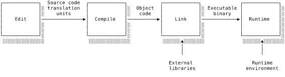
Edit time is when the developer is writing or modifying the program’s source code. Tools like linters and code formatters are able to statically analyse the source code and detect some types of errors. Here “static” means that the tool doesn’t actually execute the program. It merely analyses the source code.

The program enters compile time when it is being compiled, naturally enough. The compiler performs its own static analysis to ensure that the input is syntactically valid and well-typed. The compiler operates on chunks of code known as translation units. Depending on the language’s semantics, a translation unit might be an individual file, a class or a module. As we’ll cover in detail below, the compiler builds up an in-memory representation of the input’s structure and semantics and generates suitable output code (e.g. object code, bytecode). Depending on the semantics of the language (particularly its type system), the compiler may be able to detect many bugs at this stage including invalid syntax, incorrect types or even more subtle bugs such as non-exhaustive handling of case statements.

By itself object code can’t be directly executed. Each blob of object code is just a sequence of machine code instructions implementing the required functionality. If the code references other functions, global variables and so on, the executable code will need to know how to find them. For example, if I import a function from another translation unit, the object code will contain references to the function but will not have the function’s code or the address of its implementation. At link time a program known as the linker combines the individual blobs of object code into one, coherent executable bundle. It will lay out the object code blobs and write in missing addresses. Often the linker is a different program but is invoked automatically by the compiler. Linking is a fairly mechanical process, so we won’t look at it in great detail.

There are different ways of handling linking. Static linking is where the linker copies library functions into the binary. The Go compiler statically links the entire Go runtime into every binary. This leads to bigger binary sizes but makes it easier to deploy the binary because it’s self-contained. Alternatively, dynamic linking defers linking until runtime. The linker relies on the OS to load the necessary libraries into memory along with the program’s binary code. A common example of this approach is the C standard library. Since the C standard library is so frequently used, it makes more sense for the OS to make one copy accessible to all programs than to duplicate it in every C binary. Dynamic linking saves on binary sizes and means that improvements in a linked library are immediately available to every program linking to that library. However, it can lead to confusing portability issues when a program is compiled against one version of the library and another one is available at runtime.

Finally, runtime is when the program is actually loaded into memory and executing. Errors occurring now need to be handled gracefully in some way or they could cause the whole program to crash. Even worse, an error might not cause a crash but instead cause incorrect behaviour, possibly propagating far from the original site of the bug. This is not ideal for anyone. The runtime environment is the available functionality not directly provided by the running program. The richness of the runtime environment depends on the language and how the program is executed. At one extreme, the runtime environment might be an entire virtual machine and its interface to the physical system. Go’s runtime provides a lot of complex functionality such as automatic memory management and cooperative goroutine scheduling. C, at the other extreme, is pretty lazy and leaves all of that work to the programmer. The C runtime is therefore just a standard library of useful functions and a little bit of platform-specific code to handle passing control to and from the kernel.

Building a compiler

It’s tempting to think of compilers as somehow magical programs that reach deep into the depths of computation itself in order to give life to our squalid source code. In reality they work just the same as any other program: they take input, process it and generate output. What is special about compilers is that their input and output are other programs. High level source code goes in one end and machine code comes out the other.

As ever in computing (and life!), when we face a complex task it is helpful to break it down into simpler sub-tasks. Compilers are generally structured as a pipeline of processing steps. Each step is responsible for a different part of the compilation process. The front end of the pipeline works directly with the incoming source code. It uses its understanding of the language’s syntax and semantics to generate a language-agnostic, compiler-specific intermediate representation (IR) of the program. The front end encodes into the IR all of the knowledge it can glean from the source code. The middle end (or optimiser) takes the IR from the front end and applies a sequence of optimisations. This is where a lot of the super cool stuff goes on. Each optimisation involves analysing the IR to find areas ripe for optimisation and then manipulating the IR into a more efficient form. The back end is responsible for converting the optimised IR into target-specific machine code.

Each pipeline step should ideally be independent of the others, communicating only by passing IR to later steps. The motivation for this architecture is not just a clean separation of concerns. Code reuse is also extremely important. Imagine that you want to compile m languages on n architectures. If each language-architecture pair needed its own compiler, you’d need to write m * n compilers. The pipeline approach avoids lots of this work. We only need to write a front end for each language and a back end for each architecture, so m + n in total. The optimising middle end can be reused by every language-architecture pair.

The LLVM compiler project is a great example of this approach. It is structured as a low level, compiling virtual machine with back ends for many targets. Using LLVM is an easy way for language designers to have their language supported on a wide range of platforms. They only need to write a single front end that compiles their language into LLVM IR to gain access to all of the optimisations and targets supported by LLVM. Innovations and improvements to LLVM benefit all languages using it.

The front end

The front end converts source code into the compiler’s IR.

The input will be a flat sequence of characters in a file. The front end first splits the character sequence into its constituent parts in a process known as lexical analysis. It then parses the input to figure out its structure. Finally it performs semantic analysis to check that the program structure makes sense according to the language’s semantics. All of the information captured by the front end is encoded into IR.

Throughout this section, I’ll demonstrate how these processes work on a fragment of JSON:

1 { "names": ["Tom", "Tim", "Tam"] }

Decoding a JSON string into an object is similar to parsing source code into IR.

Lexical analysis

The front end’s work begins with lexical analysis (also known as lexing or scanning), which is performed by the lexer. The source code input will be a long sequence of characters with no clear sub-divisions or structure. Lexical analysis is the process of breaking the input into individually meaningful units known as tokens. A token is a pair of a lexical category and an optional attribute, called a lexeme, extracted from the character sequence by pattern matching. The lexer performs tokenisation by going through the character sequence and matching the input against a list of token patterns. The output is a sequence of tokens. Here’s how our JSON example might look tokenised: